逻辑回归算法的Sklearn完整复现

1. 算法参数

在scikit-learn中，逻辑回归模型由类sklearn.linear_model.LogisticRegression实现

1.1 正则项权重

1.2 L1/L2范数

创建逻辑回归模型时，有个参数penalty，其取值为l1或l2

范数实际上是用来指定正则项的形式。

• L1范数作为正则项，会让模型参数θ稀疏化，即让模型参数向量里为0的元素尽量多。
• L2范数是想成本函数中添加正则项，目的是让模型参数尽量小，但不会为0，让每个特征对预测值都有小的贡献

L1范数作为正则项的用途：

• 特征选择：排除掉那些对预测值没什么影响的特征，从而简化问题。解决过拟合问题的措施就是减少特征数量。
• 可解释性：只留下对预测值有重要影响的特征，这样就能很容易的解释模型的因果关系

大多数情况解决过拟合问题还是选择L2作为正则项。

2. 实例：乳腺癌检测

#载入数据
from sklearn.datasets import load_breast_cancer

cancer = load_breast_cancer()
X = cancer.data
y = cancer.target
print('data shape: {0};no.positive: {1};no.negatice: {2}'.format(
    X.shape,y[y==1].shape[0],y[y==0].shape[0]))
print(cancer.data[0])

data shape: (569, 30);no.positive: 357;no.negatice: 212
[1.799e+01 1.038e+01 1.228e+02 1.001e+03 1.184e-01 2.776e-01 3.001e-01
 1.471e-01 2.419e-01 7.871e-02 1.095e+00 9.053e-01 8.589e+00 1.534e+02
 6.399e-03 4.904e-02 5.373e-02 1.587e-02 3.003e-02 6.193e-03 2.538e+01
 1.733e+01 1.846e+02 2.019e+03 1.622e-01 6.656e-01 7.119e-01 2.654e-01
 4.601e-01 1.189e-01]

特征提取时，不妨从事物的内在逻辑关系入手，分析已有特征之间的关系，从而构造出新的特征。

回到乳腺癌数据集的特征问题，实际上它只关注其中的10个特征，然后构造出了每个特征的标准差及最大值，所以每个特征又衍生出了两个特征。

cancer.feature_names

array(['mean radius', 'mean texture', 'mean perimeter', 'mean area',
       'mean smoothness', 'mean compactness', 'mean concavity',
       'mean concave points', 'mean symmetry', 'mean fractal dimension',
       'radius error', 'texture error', 'perimeter error', 'area error',
       'smoothness error', 'compactness error', 'concavity error',
       'concave points error', 'symmetry error',
       'fractal dimension error', 'worst radius', 'worst texture',
       'worst perimeter', 'worst area', 'worst smoothness',
       'worst compactness', 'worst concavity', 'worst concave points',
       'worst symmetry', 'worst fractal dimension'], dtype='<U23')

#将数据集分成训练数据集和测试数据集
from sklearn.model_selection import train_test_split
X_train,X_test,y_train,y_test = train_test_split(X,y,test_size = 0.2)

#使用LogisticRegression模型进行训练，并计算训练数据集的评分数据和测试数据集的评分数据
from sklearn.linear_model import LogisticRegression

model = LogisticRegression()
model.fit(X_train,y_train)

train_score = model.score(X_train,y_train)
test_score = model.score(X_test,y_test)
print('train score: {train_score:.6f};test score: {test_score:.6f}'.format(
        train_score = train_score,test_score = test_score))

train score: 0.956044;test score: 0.938596


D:Anaconda3libsite-packagessklearnlinear_model\_logistic.py:763: ConvergenceWarning: lbfgs failed to converge (status=1):
STOP: TOTAL NO. of ITERATIONS REACHED LIMIT.

Increase the number of iterations (max_iter) or scale the data as shown in:
    https://scikit-learn.org/stable/modules/preprocessing.html
Please also refer to the documentation for alternative solver options:
    https://scikit-learn.org/stable/modules/linear_model.html#logistic-regression
  n_iter_i = _check_optimize_result(

#样本预测
import numpy as np

y_pred = model.predict(X_test)
print('matchs:{0}/{1}'.format(np.equal(y_pred,y_test).shape[0],y_test.shape[0]))

matchs:114/114

#预测概率：找出预测概率低于90%的样本
y_pred_proba = model.predict_proba(X_test) #计算每个测试样本的预测概率
#打印出第一个样本的数据，以便读者了解数据形式
print("sample of predict probability: {0}".format(y_pred_proba[0]))

#找出第一列，即预测为阴性的概率大于0.1的样本，保存在result里
y_pred_proba_0 = y_pred_proba[:,0] > 0.1
result = y_pred_proba[y_pred_proba_0]

#在result结果集里，找出第二列，即预测为阳性的概率大于0.1的样本
y_pred_proba_1 = result[:,1] > 0.1
print(result[y_pred_proba_1])

sample of predict probability: [0.84205429 0.15794571]
[[0.84205429 0.15794571]
 [0.57418613 0.42581387]
 [0.12547841 0.87452159]
 [0.38974917 0.61025083]
 [0.18114142 0.81885858]
 [0.53086336 0.46913664]
 [0.13076721 0.86923279]
 [0.79025588 0.20974412]
 [0.49267348 0.50732652]
 [0.87436064 0.12563936]
 [0.16471941 0.83528059]]

使用model.predict_proba()来计算概率。

2.1 模型优化

#使用Pipeline增加多项式特征
from sklearn.linear_model import LogisticRegression
from sklearn.preprocessing import PolynomialFeatures
from sklearn.pipeline import Pipeline

#增加多项式预处理
def polynomial_model(degree = 1,**kwarg):
    polynomial_features = PolynomialFeatures(degree = degree,
                                            include_bias = False)
    logistic_regression = LogisticRegression(**kwarg,max_iter=1000)
    pipeline = Pipeline([("polynomial_features",polynomial_features),
                        ("logistic_regression",logistic_regression)])
    return pipeline

#增加二阶多项式特征，创建并训练模型
import time

model = polynomial_model(degree = 2,penalty = 'l1',solver='liblinear')

start = time.perf_counter()
model.fit(X_train,y_train)

train_score = model.score(X_train,y_train)
cv_score = model.score(X_test,y_test)
print('elaspe:{0:.6f};train_score:{1:0.6f};cv_score:{2:.6f}'.format(
        time.perf_counter()-start,train_score,cv_score))

elaspe:0.353185;train_score:1.000000;cv_score:0.991228

#查看多少个特征没有被丢弃
logistic_regression = model.named_steps['logistic_regression']
print('model parameters shape:{0};count of non-zero element: {1}'.format(
        logistic_regression.coef_.shape,
        np.count_nonzero(logistic_regression.coef_)))

model parameters shape:(1, 495);count of non-zero element: 91

输入特征由30个增加到了495个，只保留了96个有效特征。

2.2 学习曲线

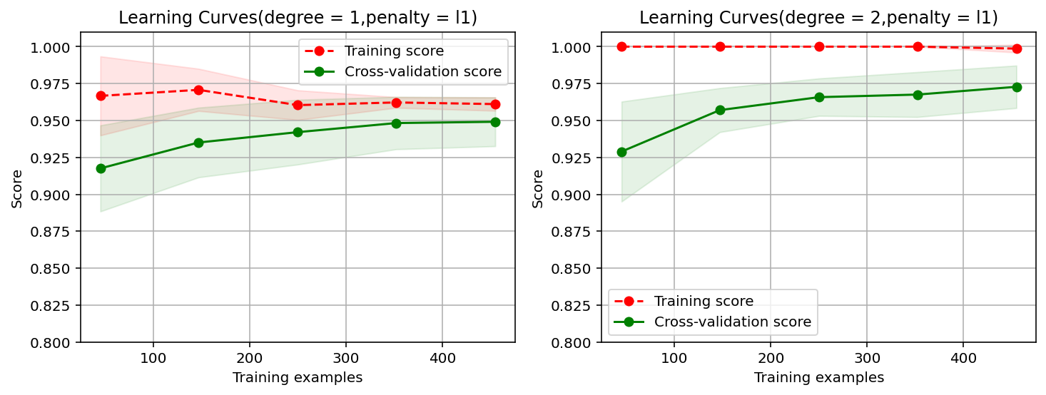
#画出L1范数作为正则项所对应的一阶和二阶多项式的学习曲线
from common.utils import plot_learning_curve
from sklearn.model_selection import ShuffleSplit
import matplotlib.pyplot as plt

cv = ShuffleSplit(n_splits = 10,test_size = 0.2,random_state = 0)
title = 'Learning Curves(degree = {0},penalty = {1})'
degrees = [1,2]
penalty = 'l1'

start = time.perf_counter()
plt.figure(figsize = (12,4),dpi = 144)
for i in range(len(degrees)):
    plt.subplot(1,len(degrees),i+1)
    plot_learning_curve(plt,
                        polynomial_model(degree=degrees[i],penalty = penalty,solver='liblinear'),
                        title.format(degrees[i],penalty),
                        X,
                        y,
                        ylim=(0.8,1.01),
                        cv = cv)
    print('elaspe:{0:.6f}'.format(time.perf_counter()-start))

elaspe:5.302274
elaspe:12.455966

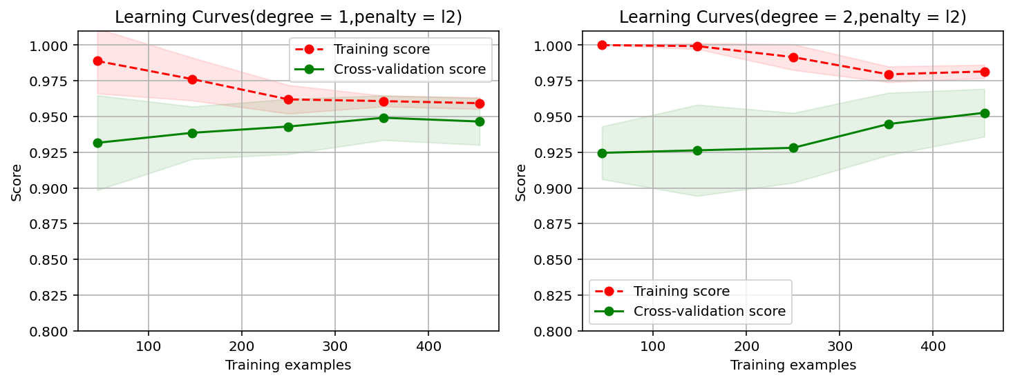
#使用L2范数作为正则项对应的一阶和二阶多项式的学习曲线
import warnings

warnings.filterwarnings("ignore")  # 忽略版本问题
penalty = 'l2'
plt.figure(figsize = (12,4),dpi = 144)
for i in range(len(degrees)):
    plt.subplot(1,len(degrees),i+1)
    plot_learning_curve(plt,
                        polynomial_model(degree=degrees[i],penalty = penalty,solver = 'lbfgs'),
                        title.format(degrees[i],penalty),
                        X,
                        y,
                        ylim=(0.8,1.01),
                        cv = cv)
    print('elaspe:{0:.6f}'.format(time.perf_counter()-start))

elaspe:224.511121
elaspe:234.462813