前言
上一篇:从零开始Pytorch-YOLOv3【笔记】(二)解析配置文件
上一篇中,我们实现了 YOLO 架构中使用的层。这一篇,我们计划用 PyTorch 实现 YOLO 网络架构,实现网络的前向传播,这样我们就能生成给定图像的输出了。
对应从零开始PyTorch项目:YOLO v3目标检测实现中的第三部分 实现网络的前向传播
定义网络
如前所述,我们使用 nn.Module 在 PyTorch 中构建自定义架构。这里,我们可以为检测器定义一个网络。在 darknet.py 文件中,我们添加了以下类:
class Darknet(nn.Module):
    def __init__(self, cfgfile):
        super(Darknet, self).__init__()
        self.blocks = parse_cfg(cfgfile)
        self.net_info, self.module_list = create_modules(self.blocks)
这里我们命名自己的model为Darknet继承nn.Moudle。我们用 members、blocks、net_info 和 module_list 对网络进行初始化。
实现网络的前向传播
该网络的前向传播通过覆写 nn.Module 类别的 forward 方法而实现。
forward 主要有两个目的。一,计算输出;二,尽早处理的方式转换输出检测特征图(例如转换之后,这些不同尺度的检测图就能够串联,不然会因为不同维度不可能实现串联)。
def forward(self, x, CUDA):
      modules = self.blocks[1:]  # self.blocks 的第一个元素是一个 net 块,它不属于前向传播。
      outputs = {}   #We cache the outputs for the route layer  由于路由层和捷径层需要之前层的输出特征图,我们在字典 outputs 中缓存每个层的输出特征图。关键在于层的索引,且值对应特征图。

      write = 0
      for i, module in enumerate(modules):
          module_type = (module["type"])

          if module_type == "convolutional" or module_type == "upsample":
              x = self.module_list[i](x)

          elif module_type == "route":
              layers = module["layers"]
              layers = [int(a) for a in layers]

              if (layers[0]) > 0:
                  layers[0] = layers[0] - i

              if len(layers) == 1:
                  x = outputs[i + (layers[0])]  # 前面某一层的tensor张量

              else:
                  if (layers[1]) > 0:
                      layers[1] = layers[1] - i

                  map1 = outputs[i + layers[0]]
                  map2 = outputs[i + layers[1]]
                  x = torch.cat((map1, map2), 1)  # 按深度拼接tensor张量


          elif  module_type == "shortcut":
              from_ = int(module["from"])
              x = outputs[i-1] + outputs[i+from_]  # 相同维度的特征图相同坐标的值相加

          elif module_type == 'yolo':
              anchors = self.module_list[i][0].anchors
              #Get the input dimensions
              inp_dim = int (self.net_info["height"])

              #Get the number of classes
              num_classes = int (module["classes"])

              #Transform
              x = x.data
              x = predict_transform(x, inp_dim, anchors, num_classes, CUDA)
              if not write:              #if no collector has been intialised.
                  detections = x
                  write = 1

              else:
                  detections = torch.cat((detections, x), 1)

          outputs[i] = x

      return detections
路由层
当moudle_type='router'路由层时,如果layer是两个参数,使用torch.cat对两个tensor张量进行拼接。第二个参数设为 1。这是因为我们希望将特征图沿深度级联起来。(在 PyTorch 中,卷积层的输入和输出的格式为B X C X H X W。深度对应通道维度batch_size,channel,height(二维数据的行数),width(二维数据的列数))。
torch.cat示例:
点击查看代码
>>> import torch
>>> A=torch.ones(2,3) #2x3的张量(矩阵)
>>> A
tensor([[ 1.,  1.,  1.],
        [ 1.,  1.,  1.]])
>>> B=2*torch.ones(4,3)#4x3的张量(矩阵)
>>> B
tensor([[ 2.,  2.,  2.],
        [ 2.,  2.,  2.],
        [ 2.,  2.,  2.],
        [ 2.,  2.,  2.]])
>>> C=torch.cat((A,B),0)#按维数0(行)拼接
>>> C
tensor([[ 1.,  1.,  1.],
         [ 1.,  1.,  1.],
         [ 2.,  2.,  2.],
         [ 2.,  2.,  2.],
         [ 2.,  2.,  2.],
         [ 2.,  2.,  2.]])
>>> C.size()
torch.Size([6, 3])
>>> D=2*torch.ones(2,4) #2x4的张量(矩阵)
>>> C=torch.cat((A,D),1)#按维数1(列)拼接
>>> C
tensor([[ 1.,  1.,  1.,  2.,  2.,  2.,  2.],
        [ 1.,  1.,  1.,  2.,  2.,  2.,  2.]])
>>> C.size()
torch.Size([2, 7])
捷径层
当moudle_type='shotcut'捷径层时,两特征图相加示例:
点击查看代码
>>> A=torch.ones(2,3)
>>> A
tensor([[1., 1., 1.],
        [1., 1., 1.]])
>>> B=2*torch.ones(2,3)
>>> B
tensor([[2., 2., 2.],
        [2., 2., 2.]])
>>> A + B
tensor([[3., 3., 3.],
        [3., 3., 3.]])

// -----如果两个张量维度不同,相加会报错----- //
>>> B=2*torch.ones(4,3)
>>> B
tensor([[2., 2., 2.],
        [2., 2., 2.],
        [2., 2., 2.],
        [2., 2., 2.]])
>>> A + B
Traceback (most recent call last):
  File "<stdin>", line 1, in <module>
RuntimeError: The size of tensor a (2) must match the size of tensor
b (4) at non-singleton dimension 0
YOLO层
这一部分建议结合从零开始PyTorch项目:YOLO v3目标检测实现中的什么是YOLO?部分一起看。
当moudle_type='yolo'YOLO层时,我们在前面知道YOLO层前的最后一层卷层使用1*1的卷积,filters=255。(classes+1+coords)*anchors_num=(5+1+80)*3=255然后YOLO层的predict_transform()方法将最后一层的卷积输出格式转换为我们可以理解的数据。
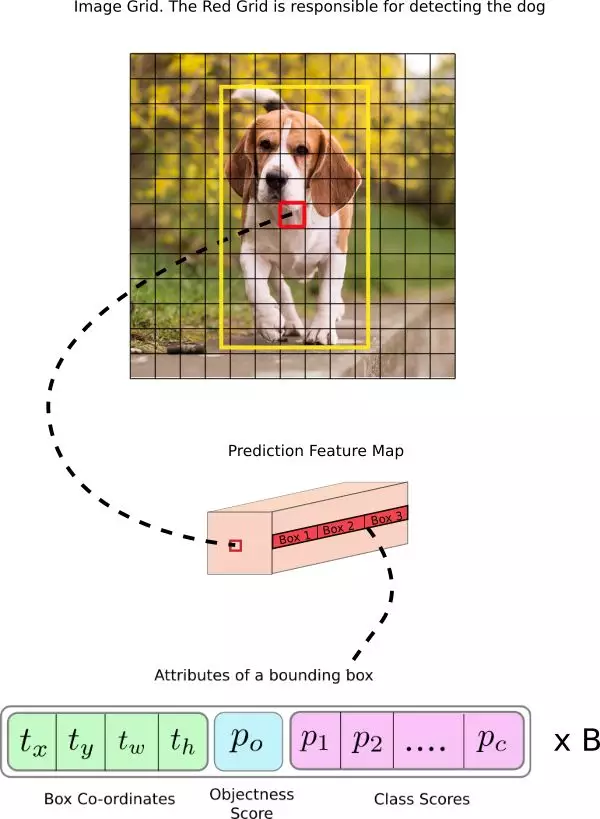
解释输出
对于一般的目标检测器来说,卷积层所学习的特征会被传递到分类器/回归器,从而进行预测(边界框的坐标、类别标签等)。YOLO是全卷积网络,没有用分类器/回归器等。通过如下方式进行解释预测。
表1是FCN全卷积网络得到的最后的feature map,我们通过predict_transform()方法转成Tensor[batch_size, grid_size*grid_size*num_anchors, bbox_attrs]的格式。其中,box_attrs=[x,y,h,w,cls,...]
predict_transform()方法: 该方法从feature map中得到了我们对边界框的预测结果。
点击查看代码
def predict_transform(prediction, inp_dim, anchors, num_classes, CUDA = True):
    '''
    Args:
        prediction: 我们的输出`(B, C, H, W)`
        inp_dim: 输入图像的维度
        anchors:
        num_classes:
        CUDA(Option): flag
    '''


    batch_size = prediction.size(0)
    stride =  inp_dim // prediction.size(2)
    grid_size = inp_dim // stride
    bbox_attrs = 5 + num_classes
    num_anchors = len(anchors)

    prediction = prediction.view(batch_size, bbox_attrs*num_anchors, grid_size*grid_size)  # 将prediction进行Reshape
    prediction = prediction.transpose(1,2).contiguous()  # transpose是二维张量的转置函数,contiguous是用于张量操作后将张量放入连续的内存中(Tensor.view就必须对连续内存的张量操作)
    # Tensor[batch_size, grid_size*grid_size, bbox_attrs*num_anchors]
    # --Reshape-->
    # Tensor[batch_size, grid_size*grid_size*num_anchors, bbox_attrs]
    prediction = prediction.view(batch_size, grid_size*grid_size*num_anchors, bbox_attrs)
    anchors = [(a[0]/stride, a[1]/stride) for a in anchors]

    #Sigmoid the  centre_X, centre_Y. and object confidencce
    # box_attrs=[x,y,h,w,cls,...]
    prediction[:,:,0] = torch.sigmoid(prediction[:,:,0])  # x,y进行归一化后,加上对应x_y_offset的值详见下面的中心坐标部分
    prediction[:,:,1] = torch.sigmoid(prediction[:,:,1])
    prediction[:,:,4] = torch.sigmoid(prediction[:,:,4])

    #Add the center offsets
    grid = np.arange(grid_size)
    a,b = np.meshgrid(grid, grid)  # Tensor.meshgrid 通俗理解:https://zhuanlan.zhihu.com/p/41968396

    x_offset = torch.FloatTensor(a).view(-1,1)
    y_offset = torch.FloatTensor(b).view(-1,1)

    if CUDA:
        x_offset = x_offset.cuda()
        y_offset = y_offset.cuda()

    x_y_offset = torch.cat((x_offset, y_offset), 1).repeat(1,num_anchors).view(-1,2).unsqueeze(0)

    prediction[:,:,:2] += x_y_offset

    # ★★★ log space transform height and the width
    anchors = torch.FloatTensor(anchors)

    if CUDA:
        anchors = anchors.cuda()

    anchors = anchors.repeat(grid_size*grid_size, 1).unsqueeze(0)
    prediction[:,:,2:4] = torch.exp(prediction[:,:,2:4])*anchors

    prediction[:,:,5: 5 + num_classes] = torch.sigmoid((prediction[:,:, 5 : 5 + num_classes]))

    prediction[:,:,:4] *= stride

    return prediction
锚点框(Anchor box)
对Anchor box的宽高进行预测会给训练带来不稳定的梯度。因此,现在绝大多是检测器都是log-space transform或者预测与anchor box直接的offset。然后,这些变换被应用到锚点框来获得预测。YOLO v3 有三个锚点,所以每个单元格会预测 3 个边界框。
预测
下面的公式描述了网络输出是如何转换,以获得边界框预测结果的。
网络为每个边界框预测4个坐标,tx,ty,tw,th。如果单元格从图像的左上角偏移(Cx,Cy),并且之前的边界框具有宽度和高度pw,ph,则相应的预测结果为:
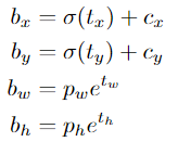
中心坐标
注意:我们使用 sigmoid 函数进行中心坐标预测。这使得输出值在 0 和 1 之间。原因如下:
正常情况下,YOLO 不会预测边界框中心的确切坐标。它预测:
-
与预测目标的网格单元左上角相关的偏移;
-
使用特征图单元的维度(1)进行归一化的偏移。
以我们的图像为例。如果中心的预测是 (0.4, 0.7),则中心在 13 x 13 特征图上的坐标是 (6.4, 6.7)(红色单元的左上角坐标是 (6,6))。
但是,如果预测到的 x,y 坐标大于 1,比如 (1.2, 0.7)。那么中心坐标是 (7.2, 6.7)。注意该中心在红色单元右侧的单元中,或第 7 行的第 8 个单元。这打破了 YOLO 背后的理论,因为如果我们假设红色框负责预测目标狗,那么狗的中心必须在红色单元中,不应该在它旁边的网格单元中。
因此,为了解决这个问题,我们对输出执行 sigmoid 函数,将输出压缩到区间 0 到 1 之间,有效确保中心处于执行预测的网格单元中。
我们对输出执行对数空间变换,然后乘锚点,来预测边界框的维度。检测器输出在最终预测之前的变换过程如图所示。
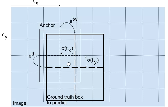
得出的预测 bw 和 bh 使用图像的高和宽进行归一化。即,如果包含目标(狗)的框的预测 bx 和 by 是 (0.3, 0.8),那么 13 x 13 特征图的实际宽和高是 (13 x 0.3, 13 x 0.8)。
变换输出格式后,将三个不同尺度的数据合并。(必须在变换后才能合并,变换之前不同尺度的feature map维度不同,不能合并。)
代码中通过设置
write=0为锚点,对三个不同尺度的变换后的数据进行合并
write = 0
for i, module in enumerate(modules):
    module_type = (module["type"])
    ...
    elif module_type == 'yolo':
      ...
      #Transform
      x = x.data
      x = predict_transform(x, inp_dim, anchors, num_classes, CUDA)
      if not write:              #if no collector has been intialised.
          detections = x
          write = 1

      else:
          detections = torch.cat((detections, x), 1)  # 将三个不同尺度的检测图级联成一个大的张量。

...

return detections
测试前向传播
下面的函数将创建一个伪造的输入,我们可以将该输入传入我们的网络。在写该函数之前,我们可以使用以下命令行将这张图像保存到工作目录:
wget https://github.com/ayooshkathuria/pytorch-yolo-v3/raw/master/dog-cycle-car.png
也可以直接下载图像:https://github.com/ayooshkathuria/pytorch-yolo-v3/raw/master/dog-cycle-car.png
现在,在 darknet.py 文件的顶部定义以下函数:
def get_test_input():
   img = cv2.imread("dog-cycle-car.png")
   img = cv2.resize(img, (416,416)) #Resize to the input dimension
   img_ = img[:,:,::-1].transpose((2,0,1)) # BGR -> RGB | H X W C -> C X H X W
   img_ = img_[np.newaxis,:,:,:]/255.0 #Add a channel at 0 (for batch) | Normalise
   img_ = torch.from_numpy(img_).float() #Convert to float
   img_ = Variable(img_) # Convert to Variable
   return img_
然后再在最后测试一下前向传播
if __name__ == '__main__':
    model = Darknet("cfg/yolov3.cfg")
    inp = get_test_input()
    pred = model(inp, not torch.cuda.is_available())  # 这里没有用GPU
    print (pred)
    print(pred.size())
报错
farward缺少一个required args CUDA
Traceback (most recent call last):
  File "d:\workspaces\YoloV3\darknet.py", line 245, in <module>
      pred = model(inp)
  File "D:\Anaconda3\envs\pytorch\lib\site-packages\torch\nn\modules\module.py", line 727, in _call_impl
      result = self.forward(*input, **kwargs)
TypeError: forward() missing 1 required positional argument: 'CUDA'
中文教程里model(imp)只有一个参数。。。加上CUDA即可。
数据一个在cpu,一个在GPU
解决方法见这篇文章:如何解决RuntimeError: Expected all tensors to be on the same device, but found at least two devices, cpu
使用is_cuda方法去判断数据在CPU还是在GPU上。
  File "d:\workspaces\YoloV3\util.py", line 91, in predict_transform
    prediction[:,:,:2] += x_y_offset
RuntimeError: Expected all tensors to be on the same device, but found at least  least two devices, cuda:0 and cpu!
在这一行前面添加
print(prediction[:,:,:2].is_cuda, x_y_offset.is_cuda)
结果是False True数据一个在cpu,一个在GPU上。那既然如此就暂且不使用GPU了,使用not torch.cuda.is_available(),cpu运行计算。
完美解决办法:原作者应该就是用的CPU测试的,其实这个网络并不大,只用CPU也就可以了。在做到第五部分,设计输入输出流程时,发现原来我的model没有运行在GPU上,所以测试代码改成如下形式,无论是CPU还是GPU就都没有问题了!!!(我们测试输入的数据也要判断一下要不要放到GPU上)
if __name__ == '__main__':
    CUDA = torch.cuda.is_available()
    model = Darknet("cfg/yolov3.cfg")
    model.load_weights("yolov3.weights")
    inp = get_test_input()
    if CUDA:
        model.cuda()
        inp = inp.cuda()
    pred = model(inp, CUDA)
    print (pred)
    print(pred.size())
输出
你将看到如下输出:
tensor([[[1.9840e+01, 1.6730e+01, 5.8778e+01,  ..., 3.8950e-01,
          6.0142e-01, 5.6941e-01],
         [1.4113e+01, 1.5334e+01, 1.2109e+02,  ..., 5.0907e-01,
          3.9206e-01, 4.7007e-01],
         [1.3489e+01, 1.5648e+01, 4.6157e+02,  ..., 4.8740e-01,
          4.2546e-01, 5.0970e-01],
         ...,
         [4.1209e+02, 4.1146e+02, 8.0367e+00,  ..., 6.3855e-01,
          5.2484e-01, 4.3740e-01],
         [4.1177e+02, 4.1166e+02, 1.2373e+01,  ..., 4.5338e-01,
          5.0231e-01, 5.0303e-01],
         [4.1288e+02, 4.1183e+02, 3.1495e+01,  ..., 4.3776e-01,
          4.4094e-01, 5.7042e-01]]])
torch.Size([1, 10647, 85])
张量的形状为 1×10647×85,第一个维度为批量大小,这里我们只使用了单张图像。对于批量中的图像,我们会有一个 100647×85 的表,它的每一行表示一个边界框(4 个边界框属性、1 个 objectness 分数和 80 个类别分数)。
现在,我们的网络有随机权重,并且不会输出正确的类别。我们需要为网络加载权重文件,因此可以利用官方权重文件。现在,我们的网络有随机权重,并且不会输出正确的类别。我们需要为网络加载权重文件,因此可以利用官方权重文件。
下载预训练权重
下载权重文件并放入检测器目录下,我们可以直接使用命令行下载:
wget https://pjreddie.com/media/files/yolov3.weights
也可以通过该地址下载:https://pjreddie.com/media/files/yolov3.weights
理解预训练权重
官方的权重文件是一个二进制文件,它以序列方式储存神经网络权重。
我们必须小心地读取权重,因为权重只是以浮点形式储存,没有其它信息能告诉我们到底它们属于哪一层。所以如果读取错误,那么很可能权重加载就全错了,模型也完全不能用。因此,只阅读浮点数,无法区别权重属于哪一层。因此,我们必须了解权重是如何存储的。
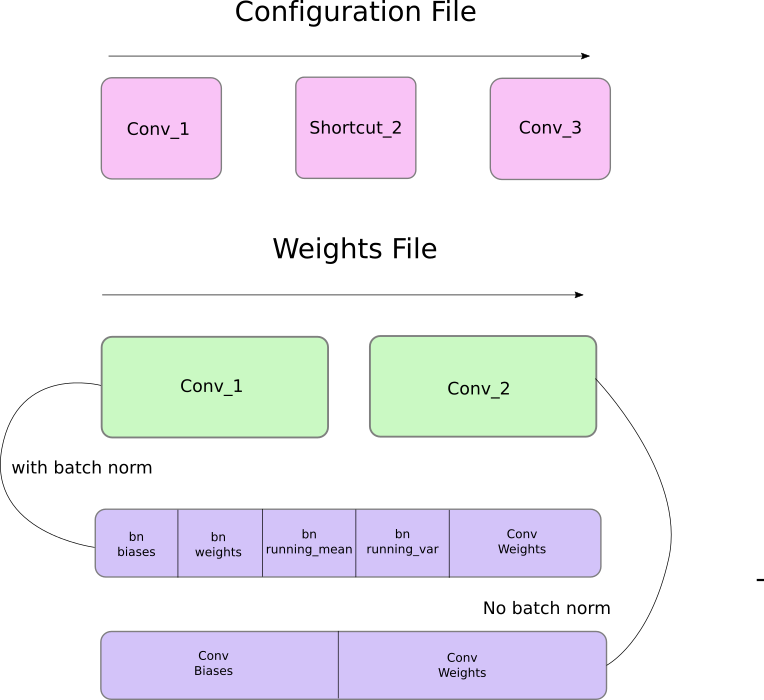
首先,权重只属于两种类型的层,即批归一化层(batch norm layer)和卷积层。这些层的权重储存顺序和配置文件中定义层级的顺序完全相同。所以,如果一个 convolutional 后面跟随着 shortcut 块,而 shortcut 连接了另一个 convolutional 块,则你会期望文件包含了先前 convolutional 块的权重,其后则是后者的权重。
当批归一化层出现在卷积模块中时,它是不带有偏置项的。然而,当卷积模块不存在批归一化,则偏置项的「权重」就会从文件中读取。下图展示了权重是如何储存的。
对应的代码:
点击查看代码
def load_weights(self, weightfile):
    #Open the weights file
    fp = open(weightfile, "rb")

    #The first 5 values are header information
    # 1. Major version number
    # 2. Minor Version Number
    # 3. Subversion number
    # 4,5. Images seen by the network (during training)
    header = np.fromfile(fp, dtype = np.int32, count = 5)  # 按类型读文件
    self.header = torch.from_numpy(header)  # torch.from_numpy()方法把数组转换成张量,且二者共享内存,对张量进行修改比如重新赋值,那么原始数组也会相应发生改变。
    self.seen = self.header[3]

    weights = np.fromfile(fp, dtype = np.float32)

    ptr = 0
    for i in range(len(self.module_list)):
        module_type = self.blocks[i + 1]["type"]

        #If module_type is convolutional load weights
        #Otherwise ignore.

        if module_type == "convolutional":
            model = self.module_list[i]
            try:
                batch_normalize = int(self.blocks[i+1]["batch_normalize"])
            except:
                batch_normalize = 0

            conv = model[0]


            if (batch_normalize):
                bn = model[1]

                #Get the number of weights of Batch Norm Layer
                num_bn_biases = bn.bias.numel()

                #Load the weights
                bn_biases = torch.from_numpy(weights[ptr:ptr + num_bn_biases])
                ptr += num_bn_biases

                bn_weights = torch.from_numpy(weights[ptr: ptr + num_bn_biases])
                ptr  += num_bn_biases

                bn_running_mean = torch.from_numpy(weights[ptr: ptr + num_bn_biases])
                ptr  += num_bn_biases

                bn_running_var = torch.from_numpy(weights[ptr: ptr + num_bn_biases])
                ptr  += num_bn_biases

                #Cast the loaded weights into dims of model weights.
                bn_biases = bn_biases.view_as(bn.bias.data)
                bn_weights = bn_weights.view_as(bn.weight.data)
                bn_running_mean = bn_running_mean.view_as(bn.running_mean)
                bn_running_var = bn_running_var.view_as(bn.running_var)

                #Copy the data to model
                bn.bias.data.copy_(bn_biases)
                bn.weight.data.copy_(bn_weights)
                bn.running_mean.copy_(bn_running_mean)
                bn.running_var.copy_(bn_running_var)

            else:
                #Number of biases
                num_biases = conv.bias.numel()

                #Load the weights
                conv_biases = torch.from_numpy(weights[ptr: ptr + num_biases])
                ptr = ptr + num_biases

                #reshape the loaded weights according to the dims of the model weights
                conv_biases = conv_biases.view_as(conv.bias.data)

                #Finally copy the data
                conv.bias.data.copy_(conv_biases)

            #Let us load the weights for the Convolutional layers
            num_weights = conv.weight.numel()

            #Do the same as above for weights
            conv_weights = torch.from_numpy(weights[ptr:ptr+num_weights])
            ptr = ptr + num_weights

            conv_weights = conv_weights.view_as(conv.weight.data)
            conv.weight.data.copy_(conv_weights)
使用
现在可以通过调用 darknet 对象上的 load_weights 函数来加载 Darknet 对象中的权重。
model = Darknet("cfg/yolov3.cfg")
    model.load_weights("yolov3.weights")
运行结果如下:
tensor([[[8.5426e+00, 1.9015e+01, 1.1130e+02,  ..., 1.7306e-03,
          1.3874e-03, 9.2985e-04],
         [1.4105e+01, 1.8867e+01, 9.4014e+01,  ..., 5.9501e-04,
          9.2471e-04, 1.3085e-03],
         [2.1125e+01, 1.5269e+01, 3.5793e+02,  ..., 8.3609e-03,
          5.1067e-03, 5.8562e-03],
         ...,
         [4.1268e+02, 4.1069e+02, 3.7157e+00,  ..., 1.7185e-06,
          4.0955e-06, 6.5897e-07],
         [4.1132e+02, 4.1023e+02, 8.0353e+00,  ..., 1.3927e-05,
          3.2252e-05, 1.2076e-05],
         [4.1076e+02, 4.1318e+02, 4.9635e+01,  ..., 4.2174e-06,
          1.0794e-05, 1.8104e-05]]])
torch.Size([1, 10647, 85])
接下来,我们将讨论使用objectness confidence thresholding和NMS产生我们的最终检测结果。