Abstract— Having dealt with a very basic local sensing based path finding algorithm -tangent bug - in the first homework, we will focus on again a very simple reactive path planning method, artificial potential fields(APF). APF is a reactive approach since the trajectories are not planned explicitly but obtained while executing actions by differentiating a function what is called potential function. A potential function is differentiable real- valued function U : Rm→ R. The output of a potential function can be taken as the energy and it’s negative gradient as the net-force acting on the robot. In this report, two different potential functions are presented; attractive-repulsive potential function, and navigation function. These two functions are tested in a simulation environment with various configurations.
Experiments are done on the robocup small-size league robot soccer platform that I have been started developing with the first homework. At the end, we see that both methods have some limitations and innate problems.
摘要——基于基础的位置感知路径规划算法——tangent bug,我们致力于一个简单的响应型路径规划方法,人工势场。人工势场是一个响应型方法,因轨迹不是精确规划,但是可以通过执行微分势函数来得到行为(指示)。势函数是可微的实数函数U : Rm→ R.势函数的输出可视作能量,他的负梯度为对机器人的场力。在这篇报告中,展示了两个不同的势函数;引力—斥力势函数,和导向函数。在模拟环境下的多种配置对这两个函数进行了测试。
在 机器人杯 小型社团机器人足球 平台上进行了实验,最后我们发现两种方法都有许多限制和内部问题。
I. Introduction
The main idea behind artificial potential field methods is finding a function that represents the energy of the system, and generating a force on the robot so that the energy of the system is minimized and reach it’s minimum value, preferably only, at the goal position.
人工势场法的主要思想是找到一个代表系统能量的函数,并且生成系统施加在机器人上的能量最小的力,并且到达系统的能量最小值(最好只有一个,在目标点)。
Therefore, moving to the goal position can be thought as moving robot from a high-value state to a low-value state by following a ”downhill” path. Mathematically speaking, this is the the process of following negative gradient, or gradient- descent, i.e. c.(t) = −∇U(c(t)). The motion terminates as soon as the gradient vanishes, that is ∇U(q∗) = 0 where q∗is called the critical value of U. This critical point is either maximum, minimum or saddle point as it shown in figure 1.Although the maximum is not that critical as soon as robot doesn’t start movement from this point, but the local minimum points are the real concern while designing a potential function. Here, one assumption is that the saddle points -being unstable points- do not cause any problem due to the robot’s inertia and other dynamics.
因此向目标点移动可被考虑成,从高水平状态向低水平状态,按照一个“下山”的路径移动机器人。用数学的语言来说,这是一个按负梯度过程,即梯度下降,也就是说 c.(t) = −∇U(c(t))。这个运动随梯度消失一起结束,也就是∇U(q∗) = 0时刻,其中q*被称作U的关键值。这个关键点是最大、最小或者马鞍点中的一个。虽然当机器人未从这个点开始移动时,不最大值不是那么关键,但是在设计势函数时,局部最小点很关键。再此,一个假说时马鞍点——作为不稳定点——不产生任何问题因为机器人的惰性和其他动态。
In this document, two main approaches, additive attractive/repulsive potential, and navigation potential functions are to be investigated. The rest of the article organized as follows: first, a brief mathematical background of potential functions are given, then the experimental framework is represented. Lastly, experimental results, pros and cons of the two methods are given in the discussion section, and it ends with conclusion.
在这篇文献中,两个主要方式,累加的引力/斥力势函数要被检测。文章的其他部分组成……
II. POTENTIAL FUNCTIONS
Two different potential functions are examined in this report, additive attractive/repulsive potential functions and navigation potential functions.
A. Additive Attractive/Repulsive Potential Functions The intuition behind the additive potential functions is attracting the robot to the goal position while repelling the robot from the obstacles by superposing these two effects into one resultant force applied on the robot. This potential function can be constructed as U(q) = Uatt(q) + Urep(q), that is the sum of the attractive and repulsive potentials.
累加的引力/斥力势函数 累加势函数背后的直觉灵感是,通过对机器人叠加这两种力,边从障碍物排斥机器人边吸引机器人到目标点。势函数构造:U(q) = Uatt(q) + Urep(q),也就是引力斥力之和
I) The Attractive Potential: The essential requirement in construction of the attractive potential is that Uatt should be monotonically increasing with the current distance d(q, qgoal) of the robot to the goal, qgoal. Two common Uatt functions are the ones having conical and/or quadratic forms.In the experiments, combinations of the two are used since the conical functions suffer from the discontinuity in the goal position, that is division-by-zero problem in computational sense.
引力场:构造引力场至关重要的是Uatt需要是随着机器人到目的地的距离 d(q, qgoal)单一增长的,两个共有的Uatt函数是由圆锥或/和二次曲线构成的。在实验中,两种结合使用,因为圆锥函数在终点不连续,在计算中会出现除零错误。
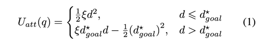
where d = d(q, qqoal), ξ is the attraction gain, and d* goal is the threshold after which quadratic function changes to the conical form.
其中d = d(q, qqoal),ξ是引力获得,d* goal 是二次曲线和圆锥的切换阈值。
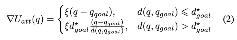
The gradient of the function (1) is obtained as;
函数(1)的梯度为
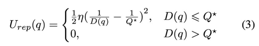
2) The Repulsive Potential: The behavior of a proper repulsive potential function should look like the behavior of a tightened spring, or the magnets getting closer to each other so that obstacle avoidance can be satisfied. In this study following formula is utilized,
斥力场:一个合适斥力势函数应该看起来像一个压紧的弹簧,或者是相互吸引的磁铁,故就可以避开障碍。在这篇研究中使用下述方程,
Derivative of the repulsive potential function(3) is the repulsive force which is
对斥力势函数求导,得到斥力
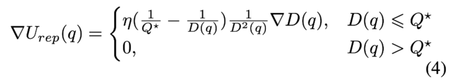
Where Q* is the distance threshold for an obstacle to create a repulsion effect on the robot, and η is the repulsion gain.
其中Q*是障碍对机器人产生斥力的阈值,η是斥力获得。
The gain parameters (i.e. η and ξ) and the threshold parameters(i.e. Q*and d*) are set empirically.The total repulsive potential field can be obtained by summing up the potentials caused by all of the obstacles,
获得参数(η和 ξ)和其他的阈值参数(Q*和d*)是凭经验设置的。总的斥力场可以通过对所有障碍引起的力加和得到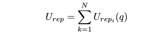
and the movement is realized by following the negative gradient of the sum of attractive/repulsive potentials or simply the following vectorial sum;
移动路径通过按照引力/斥力之和的负梯度得到,或者简单的沿着向量和移动;

In this study, the translation velocity assignment is simply done by utilizing −∇U(q)
在本研究中,速度变化的分配简单的服从负梯度−∇U(q)
B. Navigation Potential Functions Due to the local minima problem in the additive attractive/repulsive potential fields, many other local-minima free potential field methods are proposed such as wave-front planner [6][7]. However these methods have discretization problems and that’s why they become computationally intractable for high dimensional and large configuration spaces.To solve the local minima problem, a special function to be constructed which has the only minimum at the goal position.These functions are called navigation functions, formally defined in [8][9]
导向势函数 由于在累加的引力/斥力场的局部最小问题,提出了例如wave front planner等许多其他的无局部最小方法。然而这些方法有离散化问题并且就是为什么他们在高维和大规模上难以计算。为了解决局部最小的问题,构造了一个特殊的导向函数,只在终点有唯一最小值。
A function φ:Qfree → [0, 1] is called a navigation function if it
• is smooth (or at least Ckfor k>=2)
• has a unique minimum at qgoal in the connected component of the free space that contains qgoal.
• is uniformly maximal on the boundary of the free space, and
• is Morse
导向函数φ:Qfree → [0, 1]
- 平滑,或至少二阶以上可导
- 在自由空间被连接且包含qgoal的部分终点有唯一最小值
- 在自由空间边界一致最大
- Morse
As in the case of attractive/repulsive potential functions, navigation functions are used to move the robot from an arbitrary configuration to the goal configuration in the negative gradient direction of the potential at that instant. The navigation potential functions can be constructed as follows:
在引力/斥力函数的例子中,导向函数被用来沿着势场的负梯度从随机设置的起点到终点移动机器人。导向势函数构造如下:
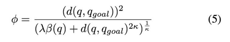
where β(q) is a repulsive-like function calculated as

for each obstacle having a radius of ri. The critical point in choosing Bi(q) is that QOi= q | βi(q) <= 0; this means βi(q) is negative inside an obstacle and it is positive outside in the free space, which requires
每个障碍物有半径 ri。选择Bi(q)的关键是 QOi= q | βi(q) <= 0;这意味着 βi(q)是在障碍物里是负值,在外部自由空间是正值。这就需要:
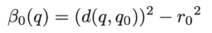
where q0 is the center and r0 is the radius of the sphere world
其中q0是中心,r0是球形空间的半径
In this report, it is assumed that the configuration space is bounded by a sphere centered at q0 and the other obstacles are also spherical centered at qi
在这篇报告中假设了设定空间被一个中心在 q0的球包围,其他的障碍也在以qi为中心的球内
The λ in the equation (5) is necessary for bounding the navigation function so that it has 0 at the goal and 1 on the boundary of any obstacle.
等式(5)中的λ对于导向函数的边界很重要,故它在终点为0,在任何障碍物的边界为1。
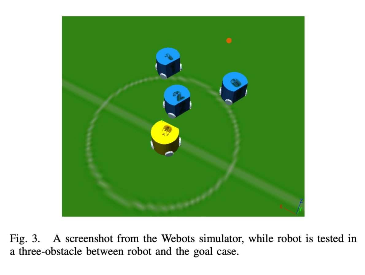
The κ on the other hand, has an effect of making the navigation function has the form of a bowl near to the goal. Increasing κ causes the other critical points(local minimum etc.) shift toward the obstacles and resulting in a negligible repulsive behavior compared to the overwhelming influence of the attractive field. The effect of increasing κ is shown in the figure2, for the case of having three obstacle in front of the robot and a goal position beyond the obstacles as it is illustrated in the figure 3.
k在另一方面,对导向函数在终点附近的碗的形状构成有影响。增加k值导致其他关键点(局部最小点等)向障碍物转移并且造成和引力场压倒的力量相比的微小的排斥行为。增加k值的影响在图2中展示,在机器人前有
三个障碍并且目的点超出障碍的情况在图3中展示。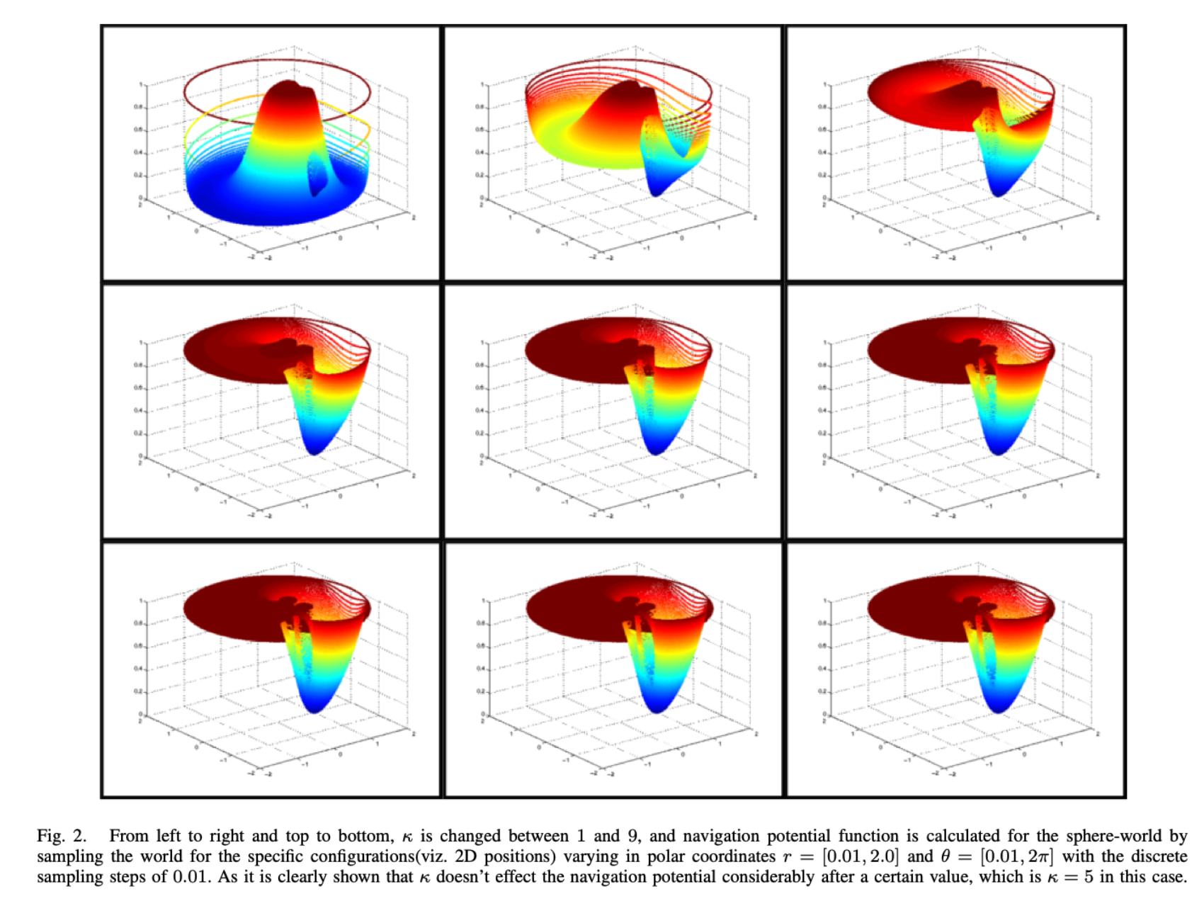
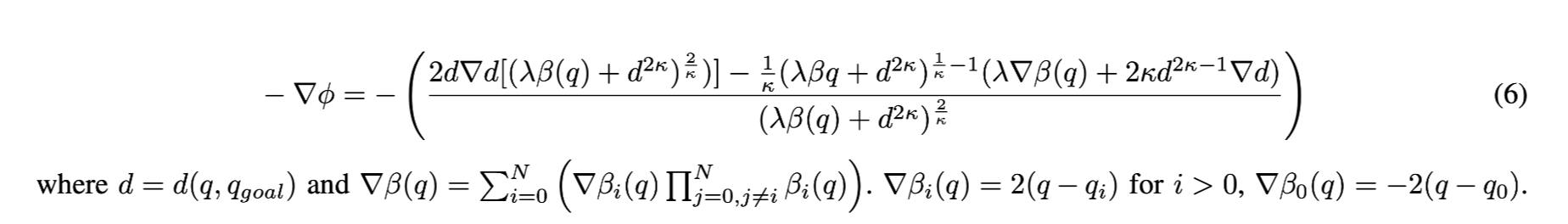
Once a ”proper” κ value is decided, robot’s configuration or -in this study- velocity is updated with the negative gradient of the navigation potential(equation (6)) function similar to the what’s been done in the attractive/repulsive potential functions.
一旦选择了适合的k值,机器人的设置,在本文中,速度随着导向场的负梯度(等式6)更新,就像之前对引力/斥力势函数做的那样。