Deep Neural Network for Image Classification: Application

来自吴恩达深度学习视频作业四 assignment4_2
如果直接看代码对你来说有困难， 请移步： https://blog.csdn.net/u013733326/article/details/79767169

import time
import numpy as np
import h5py
import matplotlib.pyplot as plt
import scipy
from PIL import Image
from scipy import ndimage
from dnn_app_utils_v2 import *

%matplotlib inline
plt.rcParams['figure.figsize'] = (5.0, 4.0) # set default size of plots
plt.rcParams['image.interpolation'] = 'nearest'
plt.rcParams['image.cmap'] = 'gray'

%load_ext autoreload
%autoreload 2

np.random.seed(1)

train_x_orig, train_y, test_x_orig, test_y, classes = load_data()

# Example of a picture
index = 7
plt.imshow(train_x_orig[index])
print ("y = " + str(train_y[0,index]) + ". It's a " + classes[train_y[0,index]].decode("utf-8") +  " picture.")

# Explore your dataset 
m_train = train_x_orig.shape[0]
num_px = train_x_orig.shape[1]
m_test = test_x_orig.shape[0]

print ("Number of training examples: " + str(m_train))
print ("Number of testing examples: " + str(m_test))
print ("Each image is of size: (" + str(num_px) + ", " + str(num_px) + ", 3)")
print ("train_x_orig shape: " + str(train_x_orig.shape))
print ("train_y shape: " + str(train_y.shape))
print ("test_x_orig shape: " + str(test_x_orig.shape))
print ("test_y shape: " + str(test_y.shape))

Number of training examples: 209
Number of testing examples: 50
Each image is of size: (64, 64, 3)
train_x_orig shape: (209, 64, 64, 3)
train_y shape: (1, 209)
test_x_orig shape: (50, 64, 64, 3)
test_y shape: (1, 50)

# Reshape the training and test examples 
train_x_flatten = train_x_orig.reshape(train_x_orig.shape[0], -1).T   # The "-1" makes reshape flatten the remaining dimensions
test_x_flatten = test_x_orig.reshape(test_x_orig.shape[0], -1).T

# Standardize data to have feature values between 0 and 1.
train_x = train_x_flatten/255.
test_x = test_x_flatten/255.

print ("train_x's shape: " + str(train_x.shape))
print ("test_x's shape: " + str(test_x.shape))

train_x's shape: (12288, 209)
test_x's shape: (12288, 50)

### CONSTANTS DEFINING THE MODEL ####
n_x = 12288     # num_px * num_px * 3
n_h = 7
n_y = 1
layers_dims = (n_x, n_h, n_y)

# GRADED FUNCTION: two_layer_model

def two_layer_model(X, Y, layers_dims, learning_rate = 0.0075, num_iterations = 3000, print_cost=False):
    """
    Implements a two-layer neural network: LINEAR->RELU->LINEAR->SIGMOID.
    
    Arguments:
    X -- input data, of shape (n_x, number of examples)
    Y -- true "label" vector (containing 0 if cat, 1 if non-cat), of shape (1, number of examples)
    layers_dims -- dimensions of the layers (n_x, n_h, n_y)
    num_iterations -- number of iterations of the optimization loop
    learning_rate -- learning rate of the gradient descent update rule
    print_cost -- If set to True, this will print the cost every 100 iterations 
    
    Returns:
    parameters -- a dictionary containing W1, W2, b1, and b2
    """
    
    np.random.seed(1)
    grads = {}
    costs = []                              # to keep track of the cost
    m = X.shape[1]                           # number of examples
    (n_x, n_h, n_y) = layers_dims
    
    # Initialize parameters dictionary, by calling one of the functions you'd previously implemented
    ### START CODE HERE ### (≈ 1 line of code)
    parameters = initialize_parameters(n_x, n_h, n_y)
    ### END CODE HERE ###
    
    # Get W1, b1, W2 and b2 from the dictionary parameters.
    W1 = parameters["W1"]
    b1 = parameters["b1"]
    W2 = parameters["W2"]
    b2 = parameters["b2"]
    
    # Loop (gradient descent)

    for i in range(0, num_iterations):

        # Forward propagation: LINEAR -> RELU -> LINEAR -> SIGMOID. Inputs: "X, W1, b1". Output: "A1, cache1, A2, cache2".
        ### START CODE HERE ### (≈ 2 lines of code)
        A1, cache1 = linear_activation_forward(X, W1, b1, "relu")
        A2, cache2 = linear_activation_forward(A1, W2, b2, "sigmoid")
        ### END CODE HERE ###
        
        # Compute cost
        ### START CODE HERE ### (≈ 1 line of code)
        cost = compute_cost(A2, Y)
        ### END CODE HERE ###
        
        # Initializing backward propagation
        dA2 = - (np.divide(Y, A2) - np.divide(1 - Y, 1 - A2))
        
        # Backward propagation. Inputs: "dA2, cache2, cache1". Outputs: "dA1, dW2, db2; also dA0 (not used), dW1, db1".
        ### START CODE HERE ### (≈ 2 lines of code)
        dA1, dW2, db2 = linear_activation_backward(dA2, cache2, "sigmoid")
        dA0, dW1, db1 = linear_activation_backward(dA1, cache1, "relu")
        ### END CODE HERE ###
        
        # Set grads['dWl'] to dW1, grads['db1'] to db1, grads['dW2'] to dW2, grads['db2'] to db2
        grads['dW1'] = dW1
        grads['db1'] = db1
        grads['dW2'] = dW2
        grads['db2'] = db2
        
        # Update parameters.
        ### START CODE HERE ### (approx. 1 line of code)
        parameters = update_parameters(parameters, grads, learning_rate)
        ### END CODE HERE ###

        # Retrieve W1, b1, W2, b2 from parameters
        W1 = parameters["W1"]
        b1 = parameters["b1"]
        W2 = parameters["W2"]
        b2 = parameters["b2"]
        
        # Print the cost every 100 training example
        if print_cost and i % 100 == 0:
            print("Cost after iteration {}: {}".format(i, np.squeeze(cost)))
        if print_cost and i % 100 == 0:
            costs.append(cost)
       
    # plot the cost

    plt.plot(np.squeeze(costs))
    plt.ylabel('cost')
    plt.xlabel('iterations (per tens)')
    plt.title("Learning rate =" + str(learning_rate))
    plt.show()
    
    return parameters
    
parameters = two_layer_model(train_x, train_y, layers_dims = (n_x, n_h, n_y), num_iterations = 2500, print_cost=True)

Cost after iteration 0: 0.6930497356599888
Cost after iteration 100: 0.6464320953428849
Cost after iteration 200: 0.6325140647912677
Cost after iteration 300: 0.6015024920354665
Cost after iteration 400: 0.5601966311605747
Cost after iteration 500: 0.5158304772764729
Cost after iteration 600: 0.4754901313943325
Cost after iteration 700: 0.4339163151225749
Cost after iteration 800: 0.4007977536203887
Cost after iteration 900: 0.3580705011323798
Cost after iteration 1000: 0.3394281538366413
Cost after iteration 1100: 0.3052753636196264
Cost after iteration 1200: 0.2749137728213015
Cost after iteration 1300: 0.24681768210614832
Cost after iteration 1400: 0.1985073503746611
Cost after iteration 1500: 0.17448318112556657
Cost after iteration 1600: 0.1708076297809737
Cost after iteration 1700: 0.113065245621647
Cost after iteration 1800: 0.09629426845937152
Cost after iteration 1900: 0.08342617959726865
Cost after iteration 2000: 0.07439078704319085
Cost after iteration 2100: 0.06630748132267933
Cost after iteration 2200: 0.059193295010381744
Cost after iteration 2300: 0.053361403485605585
Cost after iteration 2400: 0.04855478562877018

predictions_train = predict(train_x, train_y, parameters)

Accuracy: 0.9999999999999998

predictions_test = predict(test_x, test_y, parameters)

Accuracy: 0.72

### CONSTANTS ###
layers_dims = [12288, 20, 7, 5, 1] #  5-layer model
# GRADED FUNCTION: L_layer_model

def L_layer_model(X, Y, layers_dims, learning_rate = 0.0075, num_iterations = 3000, print_cost=False):#lr was 0.009
    """
    Implements a L-layer neural network: [LINEAR->RELU]*(L-1)->LINEAR->SIGMOID.
    
    Arguments:
    X -- data, numpy array of shape (number of examples, num_px * num_px * 3)
    Y -- true "label" vector (containing 0 if cat, 1 if non-cat), of shape (1, number of examples)
    layers_dims -- list containing the input size and each layer size, of length (number of layers + 1).
    learning_rate -- learning rate of the gradient descent update rule
    num_iterations -- number of iterations of the optimization loop
    print_cost -- if True, it prints the cost every 100 steps
    
    Returns:
    parameters -- parameters learnt by the model. They can then be used to predict.
    """

    np.random.seed(1)
    costs = []                         # keep track of cost
    
    # Parameters initialization.
    ### START CODE HERE ###
    parameters = initialize_parameters_deep(layers_dims)
    ### END CODE HERE ###
    
    # Loop (gradient descent)
    for i in range(0, num_iterations):

        # Forward propagation: [LINEAR -> RELU]*(L-1) -> LINEAR -> SIGMOID.
        ### START CODE HERE ### (≈ 1 line of code)
        AL, caches = L_model_forward(X, parameters)
        ### END CODE HERE ###
        
        # Compute cost.
        ### START CODE HERE ### (≈ 1 line of code)
        cost = compute_cost(AL, Y)
        ### END CODE HERE ###
    
        # Backward propagation.
        ### START CODE HERE ### (≈ 1 line of code)
        grads = L_model_backward(AL, Y, caches)
        ### END CODE HERE ###
 
        # Update parameters.
        ### START CODE HERE ### (≈ 1 line of code)
        parameters = update_parameters(parameters, grads, learning_rate)
        ### END CODE HERE ###
                
        # Print the cost every 100 training example
        if print_cost and i % 100 == 0:
            print ("Cost after iteration %i: %f" %(i, cost))
        if print_cost and i % 100 == 0:
            costs.append(cost)
            
    # plot the cost
    plt.plot(np.squeeze(costs))
    plt.ylabel('cost')
    plt.xlabel('iterations (per tens)')
    plt.title("Learning rate =" + str(learning_rate))
    plt.show()
    
    return parameters

parameters = L_layer_model(train_x, train_y, layers_dims, num_iterations = 2500, print_cost = True)

Cost after iteration 0: 0.695046
Cost after iteration 100: 0.589260
Cost after iteration 200: 0.523261
Cost after iteration 300: 0.449769
Cost after iteration 400: 0.420900
Cost after iteration 500: 0.372464
Cost after iteration 600: 0.347421
Cost after iteration 700: 0.317192
Cost after iteration 800: 0.266438
Cost after iteration 900: 0.219914
Cost after iteration 1000: 0.143579
Cost after iteration 1100: 0.453092
Cost after iteration 1200: 0.094994
Cost after iteration 1300: 0.080141
Cost after iteration 1400: 0.069402
Cost after iteration 1500: 0.060217
Cost after iteration 1600: 0.053274
Cost after iteration 1700: 0.047629
Cost after iteration 1800: 0.042976
Cost after iteration 1900: 0.039036
Cost after iteration 2000: 0.035683
Cost after iteration 2100: 0.032915
Cost after iteration 2200: 0.030472
Cost after iteration 2300: 0.028388
Cost after iteration 2400: 0.026615

pred_train = predict(train_x, train_y, parameters)

Accuracy: 0.9999999999999998

pred_test = predict(test_x, test_y, parameters)

Accuracy: 0.74

print_mislabeled_images(classes, test_x, test_y, pred_test)

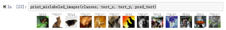
作者给出了引起判断失误的原因类型，可以作为增加新特征或改进模型的依据。

A few type of images the model tends to do poorly on include:

• Cat body in an unusual position
• Cat appears against a background of a similar color
• Unusual cat color and species
• Camera Angle
• Brightness of the picture
• Scale variation (cat is very large or small in image)

## START CODE HERE ##
my_image = "my_image2.jpg" # change this to the name of your image file 
my_label_y = [1] # the true class of your image (1 -> cat, 0 -> non-cat)
## END CODE HERE ##

fname = "images/" + my_image
image = np.array(ndimage.imread(fname, flatten=False))
my_image = scipy.misc.imresize(image, size=(num_px,num_px)).reshape((num_px*num_px*3,1))
my_predicted_image = predict(my_image, my_label_y, parameters)

plt.imshow(image)
print ("y = " + str(np.squeeze(my_predicted_image)) + ", your L-layer model predicts a "" + classes[int(np.squeeze(my_predicted_image)),].decode("utf-8") +  "" picture.")

C:UserswanghAnaconda3libsite-packagesipykernel_launcher.py:7: DeprecationWarning: `imread` is deprecated!
`imread` is deprecated in SciPy 1.0.0.
Use ``matplotlib.pyplot.imread`` instead.
  import sys
C:UserswanghAnaconda3libsite-packagesipykernel_launcher.py:8: DeprecationWarning: `imresize` is deprecated!
`imresize` is deprecated in SciPy 1.0.0, and will be removed in 1.2.0.
Use ``skimage.transform.resize`` instead.
  
Accuracy: 1.0
y = 1.0, your L-layer model predicts a "cat" picture.