目录
Tensor Flow
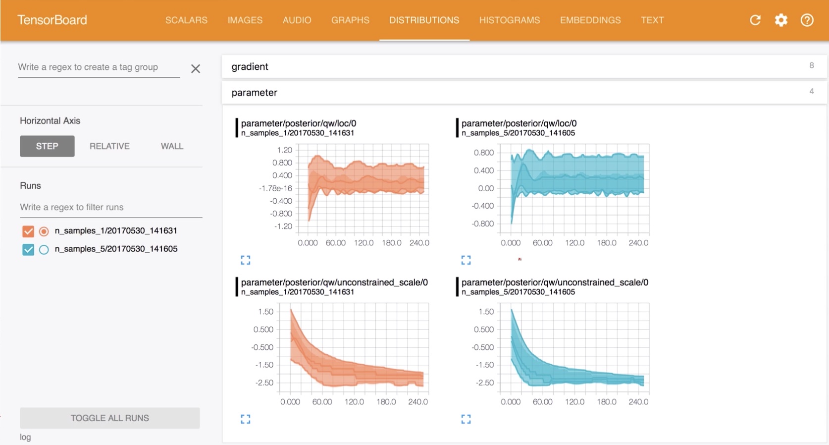
TensorBoard
-
Installation
-
Curves
-
Image Visualization
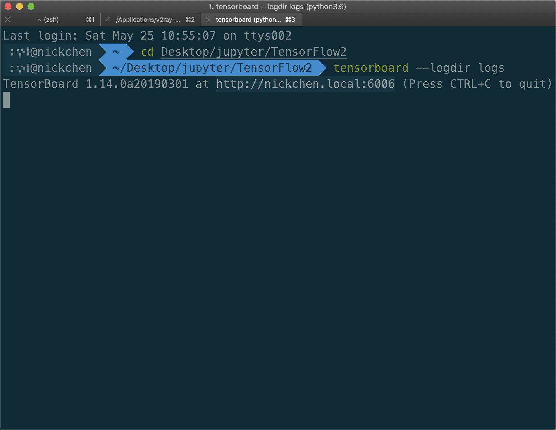
Installation
pip install tensorboard
Priciple
-
Listen logdir
-
build summary instance
-
fed data into summary instance
Step1.run listener
Step2.build summary
import datetime
import tensorflow as tf

current_time = datetime.datetime.now().strftime('%Y%m%d-%H%M%s')
log_dir = 'logs/' + current_time

summary_writer = tf.summary.create_file_writer(log_dir)
Step3.fed scalar
with summary_writer.as_default():
    tf.summary.scalar('loss', float(loss), step=epoch)
    tf.summary.scalar('accuracy', float(train_accuracy), step=epoch)
Step3.fed single Image
sample_img = next(iter(db))[0]
sample_img = sample_img[0]
sample_img = tf.reshape(sample_img, [1, 28, 28, 1])
with summary_writer.as_default():
    tf.summary.image('Traning sample:', sample_img, step=0)
Step3.fed multi-images
val_images = x[:25]
val_images = tf.reshape(val_images, [-1, 28, 28, 1])

with summary_writer.as_default():
    tf.summary.scalar('test-acc', float(loss), step=step)
    tf.summary.image('val-onebyone-images:',
                     val_images,
                     max_output=25,
                     step=step)
Instance
import tensorflow as tf
from tensorflow.keras import datasets, layers, optimizers, Sequential, metrics
import datetime
from matplotlib import pyplot as plt
import io


def preprocess(x, y):

    x = tf.cast(x, dtype=tf.float32) / 255.
    y = tf.cast(y, dtype=tf.int32)

    return x, y


def plot_to_image(figure):
    """Converts the matplotlib plot specified by 'figure' to a PNG image and
  returns it. The supplied figure is closed and inaccessible after this call."""
    # Save the plot to a PNG in memory.
    buf = io.BytesIO()
    plt.savefig(buf, format='png')
    # Closing the figure prevents it from being displayed directly inside
    # the notebook.
    plt.close(figure)
    buf.seek(0)
    # Convert PNG buffer to TF image
    image = tf.image.decode_png(buf.getvalue(), channels=4)
    # Add the batch dimension
    image = tf.expand_dims(image, 0)
    return image


def image_grid(images):
    """Return a 5x5 grid of the MNIST images as a matplotlib figure."""
    # Create a figure to contain the plot.
    figure = plt.figure(figsize=(10, 10))
    for i in range(25):
        # Start next subplot.
        plt.subplot(5, 5, i + 1, title='name')
        plt.xticks([])
        plt.yticks([])
        plt.grid(False)
        plt.imshow(images[i], cmap=plt.cm.binary)

    return figure


batchsz = 128
(x, y), (x_val, y_val) = datasets.mnist.load_data()
print('datasets:', x.shape, y.shape, x.min(), x.max())

db = tf.data.Dataset.from_tensor_slices((x, y))
db = db.map(preprocess).shuffle(60000).batch(batchsz).repeat(10)

ds_val = tf.data.Dataset.from_tensor_slices((x_val, y_val))
ds_val = ds_val.map(preprocess).batch(batchsz, drop_remainder=True)

network = Sequential([
    layers.Dense(256, activation='relu'),
    layers.Dense(128, activation='relu'),
    layers.Dense(64, activation='relu'),
    layers.Dense(32, activation='relu'),
    layers.Dense(10)
])
network.build(input_shape=(None, 28 * 28))
network.summary()

optimizer = optimizers.Adam(lr=0.01)

current_time = datetime.datetime.now().strftime("%Y%m%d-%H%M%S")
log_dir = 'logs/' + current_time
summary_writer = tf.summary.create_file_writer(log_dir)

# get x from (x,y)
sample_img = next(iter(db))[0]
# get first image instance
sample_img = sample_img[0]
sample_img = tf.reshape(sample_img, [1, 28, 28, 1])
with summary_writer.as_default():
    tf.summary.image("Training sample:", sample_img, step=0)

for step, (x, y) in enumerate(db):

    with tf.GradientTape() as tape:
        # [b, 28, 28] => [b, 784]
        x = tf.reshape(x, (-1, 28 * 28))
        # [b, 784] => [b, 10]
        out = network(x)
        # [b] => [b, 10]
        y_onehot = tf.one_hot(y, depth=10)
        # [b]
        loss = tf.reduce_mean(
            tf.losses.categorical_crossentropy(y_onehot, out,
                                               from_logits=True))

    grads = tape.gradient(loss, network.trainable_variables)
    optimizer.apply_gradients(zip(grads, network.trainable_variables))

    if step % 100 == 0:

        print(step, 'loss:', float(loss))
        with summary_writer.as_default():
            tf.summary.scalar('train-loss', float(loss), step=step)

    # evaluate
    if step % 500 == 0:
        total, total_correct = 0., 0

        for _, (x, y) in enumerate(ds_val):
            # [b, 28, 28] => [b, 784]
            x = tf.reshape(x, (-1, 28 * 28))
            # [b, 784] => [b, 10]
            out = network(x)
            # [b, 10] => [b]
            pred = tf.argmax(out, axis=1)
            pred = tf.cast(pred, dtype=tf.int32)
            # bool type
            correct = tf.equal(pred, y)
            # bool tensor => int tensor => numpy
            total_correct += tf.reduce_sum(tf.cast(correct,
                                                   dtype=tf.int32)).numpy()
            total += x.shape[0]

        print(step, 'Evaluate Acc:', total_correct / total)

        # print(x.shape)
        val_images = x[:25]
        val_images = tf.reshape(val_images, [-1, 28, 28, 1])
        with summary_writer.as_default():
            tf.summary.scalar('test-acc',
                              float(total_correct / total),
                              step=step)
            tf.summary.image("val-onebyone-images:",
                             val_images,
                             max_outputs=25,
                             step=step)

            val_images = tf.reshape(val_images, [-1, 28, 28])
            figure = image_grid(val_images)
            tf.summary.image('val-images:', plot_to_image(figure), step=step)
datasets: (60000, 28, 28) (60000,) 0 255
Model: "sequential_1"
_________________________________________________________________
Layer (type)                 Output Shape              Param #
=================================================================
dense_5 (Dense)              multiple                  200960
_________________________________________________________________
dense_6 (Dense)              multiple                  32896
_________________________________________________________________
dense_7 (Dense)              multiple                  8256
_________________________________________________________________
dense_8 (Dense)              multiple                  2080
_________________________________________________________________
dense_9 (Dense)              multiple                  330
=================================================================
Total params: 244,522
Trainable params: 244,522
Non-trainable params: 0
_________________________________________________________________
0 loss: 2.3376832008361816
0 Evaluate Acc: 0.18008814102564102
100 loss: 0.48326703906059265
200 loss: 0.25227126479148865
300 loss: 0.1876775473356247
400 loss: 0.1666598916053772
500 loss: 0.1336817890405655
500 Evaluate Acc: 0.9542267628205128
600 loss: 0.12189087271690369
700 loss: 0.1326061487197876
800 loss: 0.19785025715827942
900 loss: 0.06632998585700989
1000 loss: 0.059026435017585754
1000 Evaluate Acc: 0.96875
1100 loss: 0.1200297400355339
1200 loss: 0.20464201271533966
1300 loss: 0.07950295507907867
1400 loss: 0.13028256595134735
1500 loss: 0.0644262284040451
1500 Evaluate Acc: 0.9657451923076923
1600 loss: 0.06169471889734268
1700 loss: 0.04833034425973892
1800 loss: 0.14102090895175934
1900 loss: 0.00526371318846941
2000 loss: 0.03505736589431763
2000 Evaluate Acc: 0.9735576923076923
2100 loss: 0.08948884159326553
2200 loss: 0.035213079303503036
2300 loss: 0.15530908107757568
2400 loss: 0.13484254479408264
2500 loss: 0.17365671694278717
2500 Evaluate Acc: 0.9727564102564102
2600 loss: 0.17384998500347137
2700 loss: 0.06045734882354736
2800 loss: 0.13712377846240997
2900 loss: 0.08388100564479828
3000 loss: 0.05825091525912285
3000 Evaluate Acc: 0.9657451923076923
3100 loss: 0.08653448522090912
3200 loss: 0.06315462291240692
3300 loss: 0.05536603182554245
3400 loss: 0.2064306139945984
3500 loss: 0.043574199080467224
3500 Evaluate Acc: 0.96875
3600 loss: 0.0456567145884037
3700 loss: 0.08570165187120438
3800 loss: 0.021522987633943558
3900 loss: 0.05123775079846382
4000 loss: 0.14489373564720154
4000 Evaluate Acc: 0.9722556089743589
4100 loss: 0.08733823150396347
4200 loss: 0.04572174698114395
4300 loss: 0.06757005304098129
4400 loss: 0.018376709893345833
4500 loss: 0.024091437458992004
4500 Evaluate Acc: 0.9701522435897436
4600 loss: 0.10814780741930008
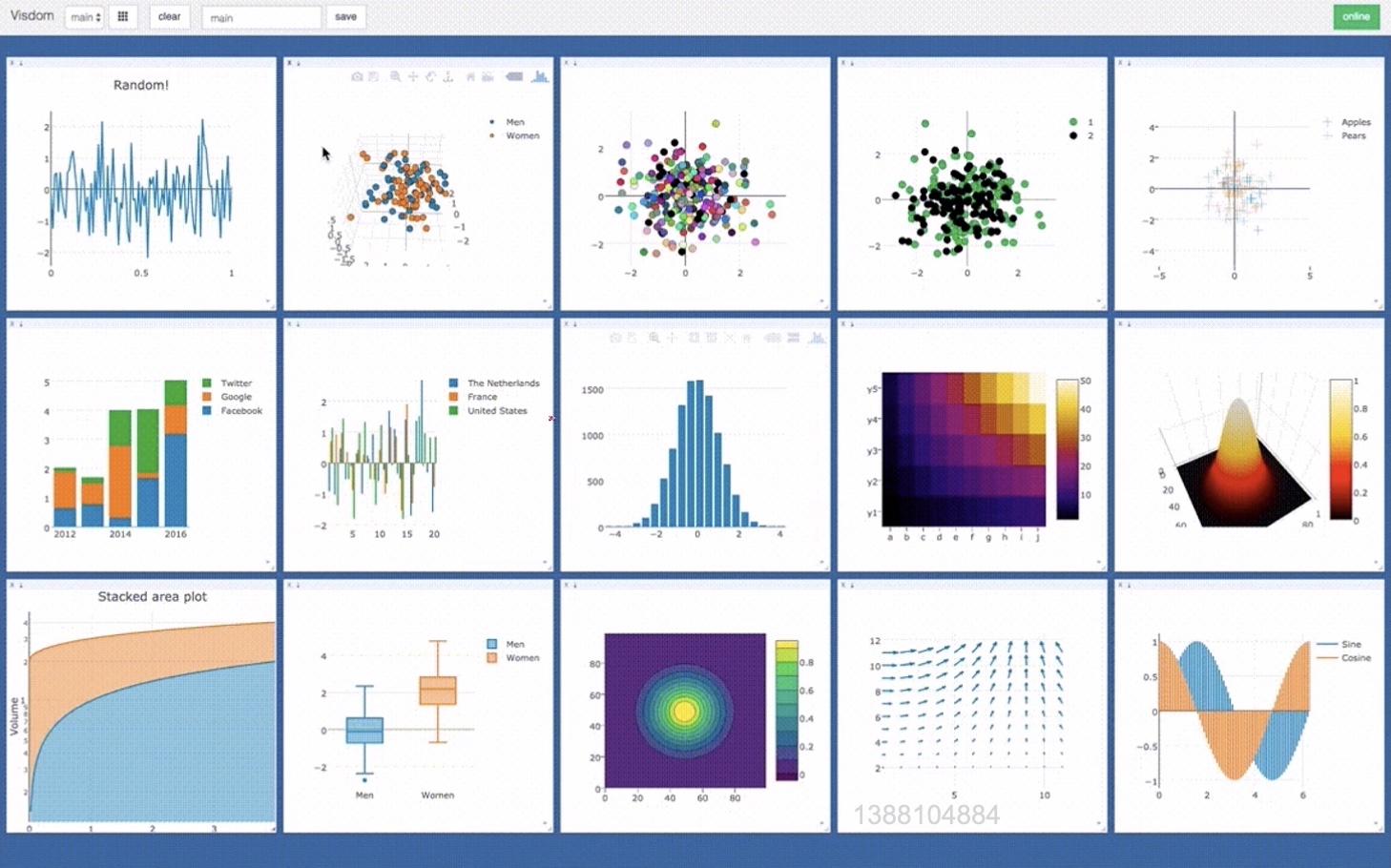
Visdom