SIFT(Scale-invariantfeature transform)是一种检测局部特征的算法,该算法通过求一幅图中的特征点(interestpoints,or corner points)及其有关scale 和 orientation 的描述子得到特征并进行图像特征点匹配,获得了良好效果,详细解析如下:
算法描述
SIFT特征不只具有尺度不变性,即使改变旋转角度,图像亮度或拍摄视角,仍然能够得到好的检测效果。整个算法分为以下几个部分:
1.构建尺度空间
高斯模糊
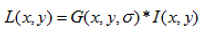
高斯核是唯一可以产生多尺度空间的核(《Scale-space theory: A basic tool for analysing structures atdifferent scales》)。一个图像的尺度空间L(x,y,σ),定义为原始图像I(x,y)与一个可变尺度的2维高斯函数G(x,y,σ)卷积运算。
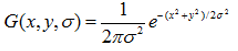
二维空间高斯函数:
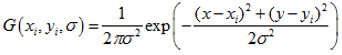
尺度空间:

尺度是自然客观存在的,不是主观创造的。高斯卷积只是表现尺度空间的一种形式。
二维空间高斯函数是等高线从中心成正太分布的同心圆:
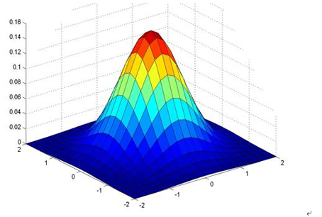
分布不为零的点组成卷积阵与原始图像做变换,即每个像素值是周围相邻像素值的高斯平均。一个5*5的高斯模版如下所示:
高斯模版是圆对称的,且卷积的结果使原始像素值有最大的权重,距离中心越远的相邻像素值权重也越小。
在实际应用中,在计算高斯函数的离散近似时,在大概3σ距离之外的像素都可以看作不起作用,这些像素的计算也就可以忽略。所以,通常程序只计算(6σ+1)*(6σ+1)就可以保证相关像素影响。
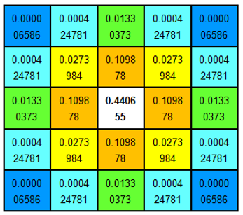
高斯模糊另一个很厉害的性质就是线性可分:使用二维矩阵变换的高斯模糊可以通过在水平和竖直方向各进行一维高斯矩阵变换相加得到。
O(N^2*m*n)次乘法就缩减成了O(N*m*n)+O(N*m*n)次乘法。(N为高斯核大小,m,n为二维图像高和宽)
高斯金字塔
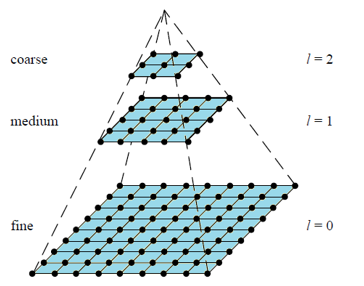
金字塔是早期图像多尺度的表示形式。图像金字塔化一般包括两个步骤:使用低通滤波器平滑图像;对平滑图像进行降采样(通常是水平,竖直方向1/2),从而得到一系列尺寸缩小的图像。
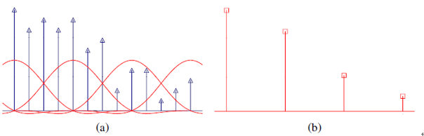
上图中(a)是对原始信号进行低通滤波,(b)是降采样得到的信号。
而对于二维图像,一个传统的金字塔中,每一层图像由上一层分辨率的长、宽各一半,也就是四分之一的像素组成:
Opencv源码:
/*
假设nOctaveLayers = 3
第0族第0幅:    sigma=1.6
第0族第1幅:    sigma=1.6   2^(1./3)*sigma
第0族第2幅:    sigma=1.6   2^(2./3)*sigma
第0族第3幅:    sigma=1.6   2^(3./3)*sigma
第0族第4幅:    sigma=1.6   2^(4./3)*sigma
第0族第5幅:    sigma=1.6   2^(5./3)*sigma
第0族-->第1族   大小变为一半   尺度为2*sigma  用的是第三幅图像的sigma
第1族第0幅:    sigma=1.6   2^(3./3)*sigma
第1族第1幅:    sigma=1.6   2^(4./3)*sigma
第1族第2幅:    sigma=1.6   2^(5./3)*sigma
第1族第3幅:    sigma=1.6   2^(6./3)*sigma
第1族第4幅:    sigma=1.6   2^(7./3)*sigma
第1族第5幅:    sigma=1.6   2^(8./3)*sigma
.....

第o族第i幅:    sigma=1.6   2^(o + i/3))*sigma
gaussian pyramid 一共有nOctaves * (nOctaveLayers + 3)幅图像

*/

void SIFT::buildGaussianPyramid( const Mat& base, vector<Mat>& pyr, int nOctaves ) const
{
    vector<double> sig(nOctaveLayers + 3);
    pyr.resize(nOctaves*(nOctaveLayers + 3));

    // precompute Gaussian sigmas using the following formula:
    //  sigma_{total}^2 = sigma_{i}^2 + sigma_{i-1}^2
	// 之所以做 sigma_{i}^2 = sigma_{total}^2 - sigma_{i-1}^2
	// 是因为每一张图像都是在上一张图像的基础上做的高斯模糊,累计起来其实就是对原始图像做了2^(o-1)*2^(n-1/nOctaveLayers)尺度的高斯模糊
    sig[0] = sigma;
    double k = pow( 2., 1. / nOctaveLayers );
    for( int i = 1; i < nOctaveLayers + 3; i++ )
    {
        double sig_prev = pow(k, (double)(i-1))*sigma;
        double sig_total = sig_prev*k;
        sig[i] = std::sqrt(sig_total*sig_total - sig_prev*sig_prev);
    }

    for( int o = 0; o < nOctaves; o++ )
    {
        for( int i = 0; i < nOctaveLayers + 3; i++ )
        {
            Mat& dst = pyr[o*(nOctaveLayers + 3) + i];
            if( o == 0  &&  i == 0 )
                dst = base;
            // base of new octave is halved image from end of previous octave
            else if( i == 0 )
            {
                const Mat& src = pyr[(o-1)*(nOctaveLayers + 3) + nOctaveLayers];
                resize(src, dst, Size(src.cols/2, src.rows/2),
                       0, 0, INTER_NEAREST);
            }
            else
            {
                const Mat& src = pyr[o*(nOctaveLayers + 3) + i-1];
                GaussianBlur(src, dst, Size(), sig[i], sig[i]);
            }
        }
    }
}
高斯金字塔的组数为:
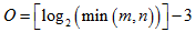
代码10-17行是计算高斯模糊的系数σ,具体关系如下:
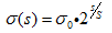
其中,σ为尺度空间坐标,s为每组中层坐标,σ0为该族中第一张图像的初始尺度,S为每组层数(一般为3~5)。根据这个公式,我们可以得到金字塔组内各层尺度以及组间各图像尺度关系。
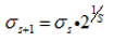
组内相邻图像尺度关系:
相邻组间尺度关系:
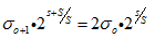
所以,相邻两组的同一层尺度为2倍的关系。
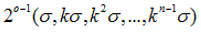
最终尺度序列总结为:
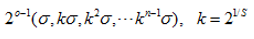
o为金字塔组数,n为每组金字塔层数。
DoG(Difference of Gaussian)差分金字塔
1)高斯拉普拉斯LoG金字塔
结合尺度空间表达和金字塔多分辨率表达,就是在使用尺度空间时使用金字塔表示,也就是计算机视觉中最有名的拉普拉斯金子塔(《The Laplacian pyramid as a compact image code》)。
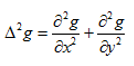
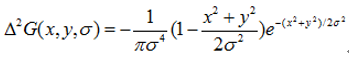
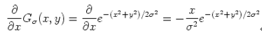
高斯拉普拉斯LoG(Laplace ofGuassian)算子就是对高斯函数进行拉普拉斯变换:
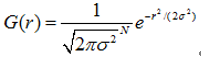
高斯核使用正太分布(高斯函数)计算模糊模版,N维空间正太分布方程为:
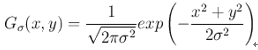
于是,二维高斯模板上的距离中心点为(x,y)的元素对应高斯计算公式为:
规范化的高斯拉普拉斯图像为
注:
高斯-拉普拉斯算法
该算法就是直接对我们的高斯模型求二阶导数
高斯卷积函数定义为:
而原始图像f(x,y) 与高斯卷积定义为:

因为:

所以Laplacian of Gaussian(LOG)可以通过先对高斯函数进行偏导操作,然后进行卷积求解。公式表示为:
和

因此,我们可以LOG核函数定义为:

最终构造LoG金字塔有5层,每层有S+2=5张图像,每层金字塔内每张图像尺度是前一张的k倍,即构成的连续尺度序列:
其中o为当前金字塔层数,n为在当前金字塔层中图像张数。
由于卷积计算性质:
******************注:两个高斯函数的卷积仍为一高斯函数(证明)****************
对于以下高斯函数 :
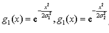
f(t)为两个高斯函数的卷积,则如下表示:
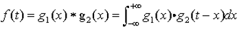
具体推导过程如下:
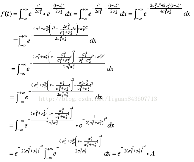
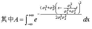
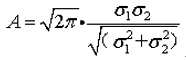
A的结果为一常数,下面给出计算过程:
运用因式替换计算,首先令 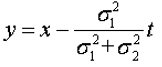

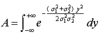
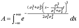
为了计算 A,将 A用另外一种形式表示:
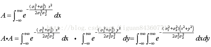
可用下式将上面的积分转换为极坐标形式:
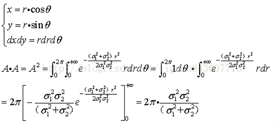
由此可知的值:
由此可得为:
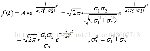
由此可知两个高斯函数的卷积为一新的高斯函数,新高斯函数的方差为原来两个高斯函数方差的和。
在计算时,通过对前一张图像做尺度系数为的卷积操作,可以减少卷积计算次数。故在金字塔每层内的S+2张图像,需要S+1次卷积操作,每次LoG核的尺度系数为:
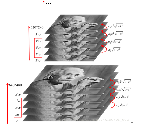
图1. LoG金字塔示意图。 左侧为图像尺度空间系数,红色矩形框为实际参与比较的空间系数,右侧为在上一张图像做LoG卷积操作的尺度系数
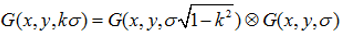
2)高斯差分DoG金字塔
DoG(Differenceof Gaussian)其实是对高斯拉普拉斯LoG的近似,也就是对的近似。SIFT算法建议,在某一尺度上的特征检测可以通过对两个相邻高斯尺度空间的图像相减,得到DoG的响应值图像D(x,y,σ)。然后仿照LoG方法,通过对响应值图像D(x,y,σ)进行局部最大值搜索,在空间位置和尺度空间定位局部特征点。其中:
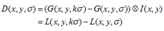
k为相邻两个尺度空间倍数的常数。
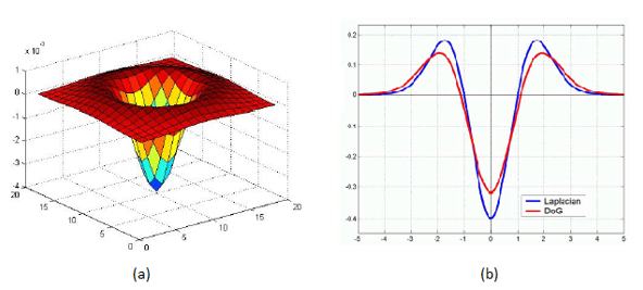
上图中(a)是DoG的三维图,(b)是DoG与LoG的对比。
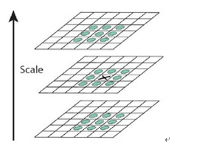
为了寻找尺度空间的极值点,每一个采样点要和它所有的相邻点比较,看其是否比它的图像域和尺度域的相邻点大或者小。如图所示,中间的检测点和它同尺度的8个相邻点和上下相邻尺度对应的9×2个点共26个点比较,以确保在尺度空间和二维图像空间都检测到极值点。一个点如果在DOG尺度空间本层以及上下两层的26个领域中是最大或最小值时,就认为该点是图像在该尺度下的一个特征点,如图所示。
同一组中的相邻尺度(由于k的取值关系,肯定是上下层)之间进行寻找
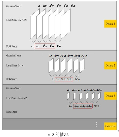
s=3的情况
在极值比较的过程中,每一组图像的首末两层是无法进行极值比较的,为了满足尺度变化的连续性(下面有详解),我们在每一组图像的顶层继续用高斯模糊生成了 3 幅图像,高斯金字塔有每组S+3层图像。DOG金字塔每组有S+2层图像。
Opencv源码:
/*
DOG Pyramid 一共有nOctaves * (nOctaveLayers + 2)幅图像
*/
void SIFT::buildDoGPyramid( const vector<Mat>& gpyr, vector<Mat>& dogpyr ) const
{
    int nOctaves = (int)gpyr.size()/(nOctaveLayers + 3);
    dogpyr.resize( nOctaves*(nOctaveLayers + 2) );

    for( int o = 0; o < nOctaves; o++ )
    {
        for( int i = 0; i < nOctaveLayers + 2; i++ )
        {
            const Mat& src1 = gpyr[o*(nOctaveLayers + 3) + i];
            const Mat& src2 = gpyr[o*(nOctaveLayers + 3) + i + 1];
            Mat& dst = dogpyr[o*(nOctaveLayers + 2) + i];
            subtract(src2, src1, dst, noArray(), DataType<sift_wt>::type);
        }
    }
}
2. 关键点搜索与定位
粗略定位:
首先通过在差分金字塔中搜寻极值点粗略在图像中寻找关键点:
寻找DoG极值点时,每一个像素点和它所有的相邻点比较,当其大于(或小于)它的图像域和尺度域的所有相邻点时,即为极值点。如下图所示,比较的范围是个3×3的立方体:中间的检测点和它同尺度的8个相邻点,以及和上下相邻尺度对应的9×2个点——共26个点比较,以确保在尺度空间和二维图像空间都检测到极值点。
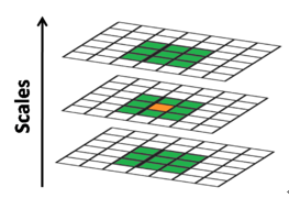
在一组中,搜索从每组的第二层开始,以第二层为当前层,第一层和第三层分别作为立方体的的上下层;搜索完成后再以第三层为当前层做同样的搜索。所以每层的点搜索两次。通常我们将组Octaves索引以-1开始,则在比较时牺牲了-1组的第0层和第N组的最高层
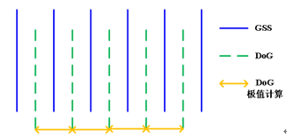
高斯金字塔,DoG图像及极值计算的相互关系如上图所示。
精确定位-----去除边缘效应
通过寻找DOG图像中的极值点能粗略找到关键点,但存在一些问题,其中之一就是DOG极值点的边缘效应,为了去除边缘效应,引入了曲率的概念。
一个平坦的DoG响应峰值在横跨边缘的地方有较大的主曲率,而在垂直边缘的地方有较小的主曲率。主曲率可以通过2×2的Hessian矩阵H求出:
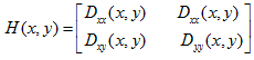
D值可以通过求临近点差分得到。H的特征值与D的主曲率成正比,具体可参见Harris角点检测算法。
注:(补充关于这里用到的部分数学知识)
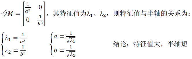
椭圆的矩阵方程表示
在高中课本中,我们学习到标准椭圆及其方程(如下图所示):
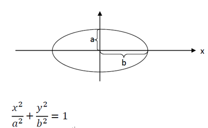
其实,矩阵在运算中使用非常广泛,现将上述标准方程写成矩阵形式(方便接下来的处理):
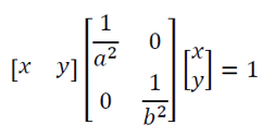
椭圆半轴与系数矩阵的关系
一个nxn的矩阵,可以求解其特征值,我们对上述系数矩阵(含a、b)进行求解,则可得到特征值与椭圆半轴(a、b)的关系,过程如下:
一元函数的泰勒展开式:
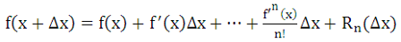
二元函数泰勒展开式:

Harris算法是利用的窗口内图像灰度的自相关性进行的,设定一个窗口,并在图像中移动,计算移动前与移动后窗口所在区域图像的自相关系数。
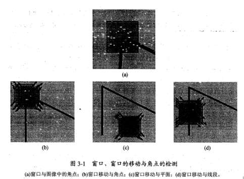
自相关函数计算如下,(x,y)为窗口中心位置,w(u,v)为权重(一般取高斯函数),L表示窗口,(u,v)表示窗口中的图像位置:
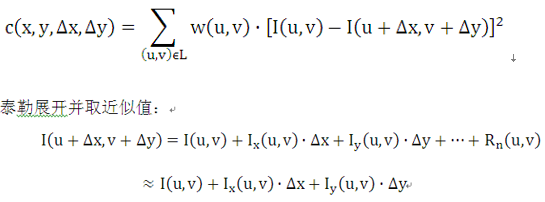
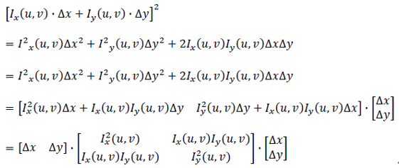
将近似值代入自相关函数,有:
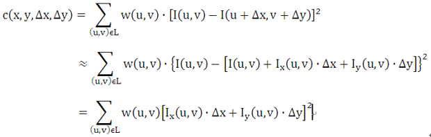
将平方项展开并写成矩阵形式,有:
回到自相关表达式:
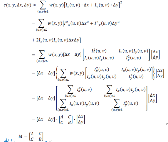
经过上面的数学形式推导,已经得到了自相关函数的表达式。可以看得这也是一个椭圆的矩阵表示形式(非标准椭圆),因此其系数矩阵M的特征值与椭圆的半轴长短有关,这与上面预备知识中的结论一样。
假设M的特征值为λ1、λ2,则分以下三种情况:
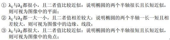
通过上面的情况,计算出特征值后就可以判别是否是角点了。
当然,这样计算量非常大,因为图像中的几乎每个点都需要进行一次特征值的计算;下面给出一个经验公式:
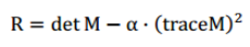
detM表示M的行列式,traceM表示M的迹,R表示角点响应值。α为经验常数,一般在0.04至0.06之间取值。
判断准则:当R超过某个设定的阈值时,可认为是角点;反之,则不是。
如此,便可得到一幅图像中的角点了,最后在3x3或5x5的邻域内进行非极大值抑制操作即可。
为了避免求具体的值,我们可以通过H将特征值的比例表示出来。令a=max lamda为最大特征值,beta=min lamda为最小特征值,那么:
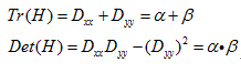
Tr(H)表示矩阵H的迹,Det(H)表示H的行列式。
令
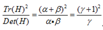
上式与两个特征值的比例有关。随着主曲率比值的增加,
精确定位-----梯度下降法确定极值点位置
通过DOG图像的26点法我们能粗略找到图像的极值点,但并不是精确的极值点,我们将粗略找到的极值点作为初始点进行迭代优化,利用二阶梯度下降法寻找精确的极值点
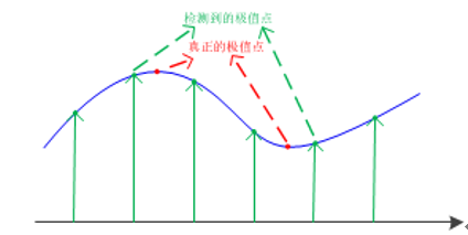
以上极值点的搜索是在离散空间进行搜索的,由下图可以看到,在离散空间找到的极值点不一定是真正意义上的极值点。可以通过对尺度空间DoG函数进行曲线拟合寻找极值点来减小这种误差。
利用DoG函数在尺度空间的Taylor展开式:
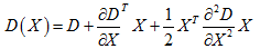
则极值点为:
程序中还除去了极值小于0.04的点。如下所示:
Opencv源码:
//
// Interpolates a scale-space extremum's location and scale to subpixel
// accuracy to form an image feature. Rejects features with low contrast.
// Based on Section 4 of Lowe's paper.
static bool adjustLocalExtrema( const vector<Mat>& dog_pyr, KeyPoint& kpt, int octv,
                                int& layer, int& r, int& c, int nOctaveLayers,
                                float contrastThreshold, float edgeThreshold, float sigma )
{
    const float img_scale = 1.f/(255*SIFT_FIXPT_SCALE);  //图像的尺度,将uchar型的图像数转化为0~1之间的图像
    const float deriv_scale = img_scale*0.5f;
    const float second_deriv_scale = img_scale;
    const float cross_deriv_scale = img_scale*0.25f;

    float xi=0, xr=0, xc=0, contr=0;
    int i = 0;

    for( ; i < SIFT_MAX_INTERP_STEPS; i++ )   //SIFT_MAX_INTERP_STEPS为迭代次数
    {
        int idx = octv*(nOctaveLayers+2) + layer;   //取该特征点所在差分金字塔的位置索引
        const Mat& img = dog_pyr[idx];
        const Mat& prev = dog_pyr[idx-1];
        const Mat& next = dog_pyr[idx+1];

        Vec3f dD((img.at<sift_wt>(r, c+1) - img.at<sift_wt>(r, c-1))*deriv_scale,
                 (img.at<sift_wt>(r+1, c) - img.at<sift_wt>(r-1, c))*deriv_scale,
                 (next.at<sift_wt>(r, c) - prev.at<sift_wt>(r, c))*deriv_scale); //分别是对x,y,z轴的差分组成的差分(微分)向量

        float v2 = (float)img.at<sift_wt>(r, c)*2;
        float dxx = (img.at<sift_wt>(r, c+1) + img.at<sift_wt>(r, c-1) - v2)*second_deriv_scale;//对x轴的二阶微分
        float dyy = (img.at<sift_wt>(r+1, c) + img.at<sift_wt>(r-1, c) - v2)*second_deriv_scale;//对y轴的二阶微分
        float dss = (next.at<sift_wt>(r, c) + prev.at<sift_wt>(r, c) - v2)*second_deriv_scale;  //对z轴的二阶微分
        float dxy = (img.at<sift_wt>(r+1, c+1) - img.at<sift_wt>(r+1, c-1) -
                     img.at<sift_wt>(r-1, c+1) + img.at<sift_wt>(r-1, c-1))*cross_deriv_scale;  //对x,y轴的分别微分
        float dxs = (next.at<sift_wt>(r, c+1) - next.at<sift_wt>(r, c-1) -
                     prev.at<sift_wt>(r, c+1) + prev.at<sift_wt>(r, c-1))*cross_deriv_scale;    //对x,z轴的分别微分
        float dys = (next.at<sift_wt>(r+1, c) - next.at<sift_wt>(r-1, c) -
                     prev.at<sift_wt>(r+1, c) + prev.at<sift_wt>(r-1, c))*cross_deriv_scale;    //对y,z轴的分别微分

        Matx33f H(dxx, dxy, dxs,
                  dxy, dyy, dys,
                  dxs, dys, dss);   //组成的海森矩阵
		//求解Hx=dD    负梯度方向(二阶梯度下降法)
        Vec3f X = H.solve(dD, DECOMP_LU);
		//梯度下降方向
        xi = -X[2];
        xr = -X[1];
        xc = -X[0];
		//设置终止条件,证明该点已经为极值点
        if( std::abs(xi) < 0.5f && std::abs(xr) < 0.5f && std::abs(xc) < 0.5f )
            break;
		//如果该点为发散的,则返回错误
        if( std::abs(xi) > (float)(INT_MAX/3) ||
            std::abs(xr) > (float)(INT_MAX/3) ||
            std::abs(xc) > (float)(INT_MAX/3) )
            return false;
		//进行梯度下降
        c += cvRound(xc);
        r += cvRound(xr);
        layer += cvRound(xi);
		//如果点坐标(x,y,z)越界 则同样返回错误
        if( layer < 1 || layer > nOctaveLayers ||
            c < SIFT_IMG_BORDER || c >= img.cols - SIFT_IMG_BORDER  ||
            r < SIFT_IMG_BORDER || r >= img.rows - SIFT_IMG_BORDER )
            return false;
    }

    // ensure convergence of interpolation  验证迭代次数没有大于最大迭代次数
    if( i >= SIFT_MAX_INTERP_STEPS )
        return false;

    {
        int idx = octv*(nOctaveLayers+2) + layer; //取该特征点所在差分金字塔的位置索引
        const Mat& img = dog_pyr[idx];
        const Mat& prev = dog_pyr[idx-1];
        const Mat& next = dog_pyr[idx+1];
        Matx31f dD((img.at<sift_wt>(r, c+1) - img.at<sift_wt>(r, c-1))*deriv_scale,
                   (img.at<sift_wt>(r+1, c) - img.at<sift_wt>(r-1, c))*deriv_scale,
                   (next.at<sift_wt>(r, c) - prev.at<sift_wt>(r, c))*deriv_scale);   //微分向量
        float t = dD.dot(Matx31f(xc, xr, xi)); //内积   将微分向量与梯度下降的方向做内积
		//????????????????????????
        contr = img.at<sift_wt>(r, c)*img_scale + t * 0.5f;
        if( std::abs( contr ) * nOctaveLayers < contrastThreshold )
            return false;

        // principal curvatures are computed using the trace and det of Hessian
		// 避免计算特征值的麻烦,海森矩阵的特征值与主曲率成正比 ,这里用Tr(H)^2/Det(H)>edgeThreshold来近似代替主曲率
		// 设a,b分别为海森矩阵特征值,则令r=a/b  Tr(H)=a+b   Det(H)=a*b   Tr(H)^2/Det(H)=(r+1)^2/r
        float v2 = img.at<sift_wt>(r, c)*2.f;
        float dxx = (img.at<sift_wt>(r, c+1) + img.at<sift_wt>(r, c-1) - v2)*second_deriv_scale;
        float dyy = (img.at<sift_wt>(r+1, c) + img.at<sift_wt>(r-1, c) - v2)*second_deriv_scale;
        float dxy = (img.at<sift_wt>(r+1, c+1) - img.at<sift_wt>(r+1, c-1) -
                     img.at<sift_wt>(r-1, c+1) + img.at<sift_wt>(r-1, c-1)) * cross_deriv_scale;
        float tr = dxx + dyy;
        float det = dxx * dyy - dxy * dxy;

        if( det <= 0 || tr*tr*edgeThreshold >= (edgeThreshold + 1)*(edgeThreshold + 1)*det )
            return false;
    }
	// 特征点的精确位置(对应原始图像的位置(x,y))
    kpt.pt.x = (c + xc) * (1 << octv);
    kpt.pt.y = (r + xr) * (1 << octv);
	// 特征点所在的族
    kpt.octave = octv + (layer << 8) + (cvRound((xi + 0.5)*255) << 16);
	// 该特征点所在的尺度大小为:该特征点所在尺度  2^(octv+layer/nOctaveLayers)*sigma  *  2 因为平时所说的尺度为半径,这里是长度
    kpt.size = sigma*powf(2.f, (layer + xi) / nOctaveLayers)*(1 << octv)*2;
    kpt.response = std::abs(contr);

    return true;
}

//
// Detects features at extrema in DoG scale space.  Bad features are discarded
// based on contrast and ratio of principal curvatures.
void SIFT::findScaleSpaceExtrema( const vector<Mat>& gauss_pyr, const vector<Mat>& dog_pyr,
                                  vector<KeyPoint>& keypoints ) const
{
	//由于gauss_pyr一共存在nOctaves*(nOctaveLayers + 3)幅图像  所以族数nOctaves = gauss_pyr.size()/(nOctaveLayers + 3);
    int nOctaves = (int)gauss_pyr.size()/(nOctaveLayers + 3);
    int threshold = cvFloor(0.5 * contrastThreshold / nOctaveLayers * 255 * SIFT_FIXPT_SCALE);
    const int n = SIFT_ORI_HIST_BINS;  //将方向分为36个bin
    float hist[n];
    KeyPoint kpt;

    keypoints.clear();

    for( int o = 0; o < nOctaves; o++ )
        for( int i = 1; i <= nOctaveLayers; i++ ) //注意这里是从第1张图像到第nOctaveLayers图像   而第0张图像和第nOctaveLayers+1张图像将不作处理,也是为什么我们要取nOctaveLayers+3张高斯图像的原因
        {
            int idx = o*(nOctaveLayers+2)+i;  //取差分金字塔当前族当前层的图像及其上一张图像和下一张图像
            const Mat& img = dog_pyr[idx];
            const Mat& prev = dog_pyr[idx-1];
            const Mat& next = dog_pyr[idx+1];
            int step = (int)img.step1();
            int rows = img.rows, cols = img.cols;

            for( int r = SIFT_IMG_BORDER; r < rows-SIFT_IMG_BORDER; r++)
            {
                const sift_wt* currptr = img.ptr<sift_wt>(r);
                const sift_wt* prevptr = prev.ptr<sift_wt>(r);
                const sift_wt* nextptr = next.ptr<sift_wt>(r);

                for( int c = SIFT_IMG_BORDER; c < cols-SIFT_IMG_BORDER; c++)
                {
                    sift_wt val = currptr[c];

                    // find local extrema with pixel accuracy  如果该点大于三维坐标系下周边所有临近的26个点,才证明该点有可能是极值点
                    if( std::abs(val) > threshold &&
                       ((val > 0 && val >= currptr[c-1] && val >= currptr[c+1] &&
                         val >= currptr[c-step-1] && val >= currptr[c-step] && val >= currptr[c-step+1] &&
                         val >= currptr[c+step-1] && val >= currptr[c+step] && val >= currptr[c+step+1] &&
                         val >= nextptr[c] && val >= nextptr[c-1] && val >= nextptr[c+1] &&
                         val >= nextptr[c-step-1] && val >= nextptr[c-step] && val >= nextptr[c-step+1] &&
                         val >= nextptr[c+step-1] && val >= nextptr[c+step] && val >= nextptr[c+step+1] &&
                         val >= prevptr[c] && val >= prevptr[c-1] && val >= prevptr[c+1] &&
                         val >= prevptr[c-step-1] && val >= prevptr[c-step] && val >= prevptr[c-step+1] &&
                         val >= prevptr[c+step-1] && val >= prevptr[c+step] && val >= prevptr[c+step+1]) ||
                        (val < 0 && val <= currptr[c-1] && val <= currptr[c+1] &&
                         val <= currptr[c-step-1] && val <= currptr[c-step] && val <= currptr[c-step+1] &&
                         val <= currptr[c+step-1] && val <= currptr[c+step] && val <= currptr[c+step+1] &&
                         val <= nextptr[c] && val <= nextptr[c-1] && val <= nextptr[c+1] &&
                         val <= nextptr[c-step-1] && val <= nextptr[c-step] && val <= nextptr[c-step+1] &&
                         val <= nextptr[c+step-1] && val <= nextptr[c+step] && val <= nextptr[c+step+1] &&
                         val <= prevptr[c] && val <= prevptr[c-1] && val <= prevptr[c+1] &&
                         val <= prevptr[c-step-1] && val <= prevptr[c-step] && val <= prevptr[c-step+1] &&
                         val <= prevptr[c+step-1] && val <= prevptr[c+step] && val <= prevptr[c+step+1])))
                    {
                        int r1 = r, c1 = c, layer = i;
						//将极值点进行差值精确找到极值点的位置,提高精度的位极值点的x,y坐标以及该极值点所处的层数layer  注意并不优化极值点所在的族数
						//并且该函数将剔除差分金字塔的边缘效应
                        if( !adjustLocalExtrema(dog_pyr, kpt, o, layer, r1, c1,
                                                nOctaveLayers, (float)contrastThreshold,
                                                (float)edgeThreshold, (float)sigma) )
                            continue;
						//计算该特征点所在层数相对于该族第0层图像的尺度比例 sigma
                        float scl_octv = kpt.size*0.5f/(1 << o);
						//计算该特征点在高斯金字塔下的方向梯度直方图
                        float omax = calcOrientationHist(gauss_pyr[o*(nOctaveLayers+3) + layer],
                                                         Point(c1, r1),
                                                         cvRound(SIFT_ORI_RADIUS * scl_octv),  //// 9sigma/2
                                                         SIFT_ORI_SIG_FCTR * scl_octv,  // 3sigma/2
                                                         hist, n);
                        float mag_thr = (float)(omax * SIFT_ORI_PEAK_RATIO);
						//将所有hist值大于主方向对应hist值得所有方向都作为特征点的方向加入特征点vector容器中  找寻辅助方向
                        for( int j = 0; j < n; j++ )
                        {
                            int l = j > 0 ? j - 1 : n - 1;
                            int r2 = j < n-1 ? j + 1 : 0;

                            if( hist[j] > hist[l]  &&  hist[j] > hist[r2]  &&  hist[j] >= mag_thr )
                            {
                                float bin = j + 0.5f * (hist[l]-hist[r2]) / (hist[l] - 2*hist[j] + hist[r2]);
                                bin = bin < 0 ? n + bin : bin >= n ? bin - n : bin;
                                kpt.angle = 360.f - (float)((360.f/n) * bin);
                                if(std::abs(kpt.angle - 360.f) < FLT_EPSILON)
                                    kpt.angle = 0.f;
                                keypoints.push_back(kpt);
                            }
                        }
                    }
                }
            }
        }
}
3. 关键点方向赋值
梯度方向和幅值
在前文中,精确定位关键点后也找到改特征点的尺度值σ,根据这一尺度值,得到最接近这一尺度值的高斯图像:
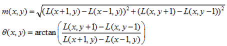
使用有限差分,计算以关键点为中心,以3×1.5σ为半径的区域内图像梯度的幅角和幅值,公式如下:
梯度直方图
在完成关键点邻域内高斯图像梯度计算后,使用直方图统计邻域内像素对应的梯度方向和幅值。
有关直方图的基础知识可以参考《数字图像直方图》,可以看做是离散点的概率表示形式。此处方向直方图的核心是统计以关键点为原点,一定区域内的图像像素点对关键点方向生成所作的贡献。
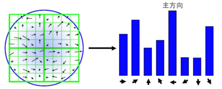
梯度方向直方图的横轴是梯度方向角,纵轴是剃度方向角对应的梯度幅值累加值。梯度方向直方图将0°~360°的范围分为36个柱,每10°为一个柱。下图是从高斯图像上求取梯度,再由梯度得到梯度方向直方图的例图。
在计算直方图时,每个加入直方图的采样点都使用圆形高斯函数函数进行了加权处理,也就是进行高斯平滑。这主要是因为SIFT算法只考虑了尺度和旋转不变形,没有考虑仿射不变性。通过高斯平滑,可以使关键点附近的梯度幅值有较大权重,从而部分弥补没考虑仿射不变形产生的特征点不稳定。
通常离散的梯度直方图要进行插值拟合处理,以求取更精确的方向角度值。(这和《关键点搜索与定位》中插值的思路是一样的)。
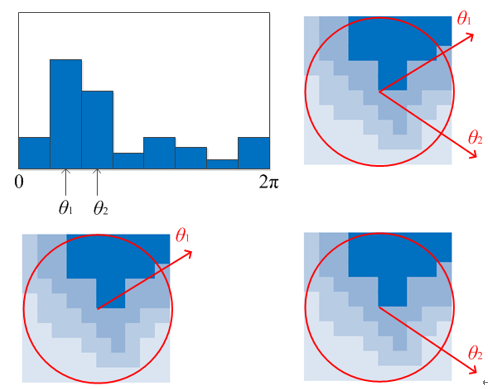
关键点方向
直方图峰值代表该关键点处邻域内图像梯度的主方向,也就是该关键点的主方向。在梯度方向直方图中,当存在另一个相当于主峰值80%能量的峰值时,则将这个方向认为是该关键点的辅方向。所以一个关键点可能检测得到多个方向,这可以增强匹配的鲁棒性。Lowe的论文指出大概有15%关键点具有多方向,但这些点对匹配的稳定性至为关键。
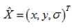
获得图像关键点主方向后,每个关键点有三个信息(x,y,σ,θ):位置、尺度、方向。由此我们可以确定一个SIFT特征区域。通常使用一个带箭头的圆或直接使用箭头表示SIFT区域的三个值:中心表示特征点位置,半径表示关键点尺度(r=2.5σ),箭头表示主方向。具有多个方向的关键点可以复制成多份,然后将方向值分别赋给复制后的关键点。如下图:
opencv源码:
// Computes a gradient orientation histogram at a specified pixel
//在高斯金字塔下计算特征点的梯度直方图
static float calcOrientationHist( const Mat& img, Point pt, int radius,
                                  float sigma, float* hist, int n )
{
    int i, j, k, len = (radius*2+1)*(radius*2+1);

    float expf_scale = -1.f/(2.f * sigma * sigma);
    AutoBuffer<float> buf(len*4 + n+4);   //为下面的变量开辟地址空间
    float *X = buf, *Y = X + len, *Mag = X, *Ori = Y + len, *W = Ori + len;
    float* temphist = W + len + 2;

    for( i = 0; i < n; i++ ) //36个bin  temphist数组存储该bin的权值
        temphist[i] = 0.f;

    for( i = -radius, k = 0; i <= radius; i++ )
    {
        int y = pt.y + i;
        if( y <= 0 || y >= img.rows - 1 )
            continue;
        for( j = -radius; j <= radius; j++ )
        {
            int x = pt.x + j;
            if( x <= 0 || x >= img.cols - 1 )
                continue;

            float dx = (float)(img.at<sift_wt>(y, x+1) - img.at<sift_wt>(y, x-1));
            float dy = (float)(img.at<sift_wt>(y-1, x) - img.at<sift_wt>(y+1, x));
			// X为每个特征点对应范围内x方向的梯度 Y对应的是每个特征点对应范围内y方向的梯度  W是每个特征点对应范围内的权值
            X[k] = dx; Y[k] = dy; W[k] = (i*i + j*j)*expf_scale;
            k++;
        }
    }

    len = k;

    // compute gradient values, orientations and the weights over the pixel neighborhood
	// 梯度的权值  根据高斯核的尺度sigma决定(半径大小)
    exp(W, W, len);
	// 梯度的幅角
    fastAtan2(Y, X, Ori, len, true);
	// 梯度的幅值
    magnitude(X, Y, Mag, len);

    for( k = 0; k < len; k++ )
    {
        int bin = cvRound((n/360.f)*Ori[k]);  //计算当前角度属于哪个bin
        if( bin >= n )
            bin -= n;
        if( bin < 0 )
            bin += n;
        temphist[bin] += W[k]*Mag[k];   //根据幅值和权重加入到该bin的方向直方图中
    }

    // smooth the histogram   对直方图进行滤波(高斯滤波)
    temphist[-1] = temphist[n-1];
    temphist[-2] = temphist[n-2];
    temphist[n] = temphist[0];
    temphist[n+1] = temphist[1];
    for( i = 0; i < n; i++ )
    {
        hist[i] = (temphist[i-2] + temphist[i+2])*(1.f/16.f) +
            (temphist[i-1] + temphist[i+1])*(4.f/16.f) +
            temphist[i]*(6.f/16.f);
    }
	//得到主方向  对应最大的值
    float maxval = hist[0];
    for( i = 1; i < n; i++ )
        maxval = std::max(maxval, hist[i]);

    return maxval;
}
4. 关键点描述
关键点描述,即用用一组向量将这个关键点描述出来,这个描述子不但包括关键点,也包括关键点周围对其有贡献的像素点。用来作为目标匹配的依据(所以描述子应该有较高的独特性,以保证匹配率),也可使关键点具有更多的不变特性,如光照变化、3D视点变化等。
SIFT描述子h(x,y,θ)是对关键点附近邻域内高斯图像梯度统计的结果,是一个三维矩阵,但通常用一个矢量来表示。矢量通过对三维矩阵按一定规律排列得到。
确定计算描述子所需的图像区域
特征描述子与特征点所在的尺度有关,因此,对梯度的求取应在特征点对应的高斯图像上进行。将关键点附近的邻域划分为d*d(Lowe建议d=4)个子区域,每个子区域做为一个种子点,每个种子点有8个方向。每个子区域的大小与关键点方向分配时相同,即每个区域有3sigma个子像素,为每个子区域分配边长为3*sigma的矩形区域进行采样(个子像素实际用边长为sqrt(3*sigma)的矩形区域即可包含,但由式(3-8),3*sigma<6sigma不大,为了简化计算取其边长为3*sigma,并且采样点宜多不宜少)。考虑到实际计算时,需要采用双线性插值,所需图像窗口边长为3*sigma*(d+1)。在考虑到旋转因素(方便下一步将坐标轴旋转到关键点的方向),如下图6.1所示,实际计算所需的图像区域半径为:
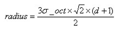
计算结果四舍五入取整。
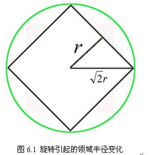
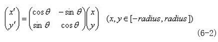
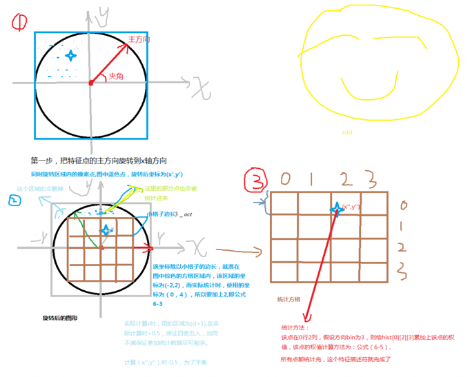
将坐标轴旋转为关键点的方向,以确保旋转不变性
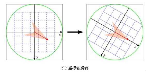
如6.2所示。 旋转后邻域内采样点的新坐标为:
将邻域内的采样点分配到对应的子区域内,将子区域内的梯度值分配到8个方向上,计算其权值。
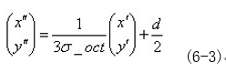
旋转后的采样点坐标在半径为radius的圆内被分配到的子区域,计算影响子区域的采样点的梯度和方向,分配到8个方向上。
旋转后的采样点落在子区域的下标为
Lowe建议子区域的像素的梯度大小按的高斯加权计算,即
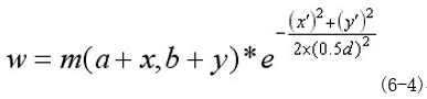
其中a,b为关键点在高斯金字塔图像中的位置坐标。
插值计算每个种子点八个方向的梯度。
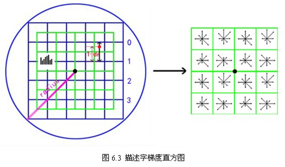
如图6.3所示,将由式(6-3)所得采样点在子区域中的下标(图中蓝色窗口内红色点)线性插值,计算其对每个种子点的贡献。如图中的红色点,落在第0行和第1行之间,对这两行都有贡献。对第0行第3列种子点的贡献因子为dr,对第1行第3列的贡献因子为1-dr,同理,对邻近两列的贡献因子为dc和1-dc,对邻近两个方向的贡献因子为do和1-do。则最终累加在每个方向上的梯度大小为:

其中k,m,n为0或为1。
如上统计的4*4*8=128个梯度信息即为该关键点的特征向量。
特征向量形成后,为了去除光照变化的影响,需要对它们进行归一化处理,对于图像灰度值整体漂移,图像各点的梯度是邻域像素相减得到,所以也能去除。得到的描述子向量为,归一化后的特征向量为则
描述子向量门限。
非线性光照,相机饱和度变化对造成某些方向的梯度值过大,而对方向的影响微弱。因此设置门限值(向量归一化后,一般取0.2)截断较大的梯度值。然后,再进行一次归一化处理,提高特征的鉴别性。
按特征点的尺度对特征描述向量进行排序。
至此,SIFT特征描述向量生成。
描述向量这块不好理解,我画了个草图,供参考:
Opencv源码:
//计算SIFT描述子
static void calcSIFTDescriptor( const Mat& img, Point2f ptf, float ori, float scl,
                               int d, int n, float* dst )
{
    Point pt(cvRound(ptf.x), cvRound(ptf.y));
    float cos_t = cosf(ori*(float)(CV_PI/180));
    float sin_t = sinf(ori*(float)(CV_PI/180));
    float bins_per_rad = n / 360.f;
    float exp_scale = -1.f/(d * d * 0.5f);
    float hist_width = SIFT_DESCR_SCL_FCTR * scl;  //3*sigma   3sigma之外的点对当前点的影响不大,关联性不大(3sigma原则)
    int radius = cvRound(hist_width * 1.4142135623730951f * (d + 1) * 0.5f);  //满足旋转型和三次线性插值 将半径变为此
    // Clip the radius to the diagonal of the image to avoid autobuffer too large exception
    radius = std::min(radius, (int) sqrt((double) img.cols*img.cols + img.rows*img.rows));
    cos_t /= hist_width;  //为了计算时y''= 1/3sigma*(j * cos_t - i * sin_t)
    sin_t /= hist_width;  //为了计算时x''= 1/3sigma*(j * sin_t + i * cos_t)

    int i, j, k, len = (radius*2+1)*(radius*2+1), histlen = (d+2)*(d+2)*(n+2);
    int rows = img.rows, cols = img.cols;

    AutoBuffer<float> buf(len*6 + histlen);
    float *X = buf, *Y = X + len, *Mag = Y, *Ori = Mag + len, *W = Ori + len;
    float *RBin = W + len, *CBin = RBin + len, *hist = CBin + len;

    for( i = 0; i < d+2; i++ )
    {
        for( j = 0; j < d+2; j++ )
            for( k = 0; k < n+2; k++ )
                hist[(i*(d+2) + j)*(n+2) + k] = 0.;
    }

    for( i = -radius, k = 0; i <= radius; i++ )
        for( j = -radius; j <= radius; j++ )
        {
            // Calculate sample's histogram array coords rotated relative to ori.
            // Subtract 0.5 so samples that fall e.g. in the center of row 1 (i.e.
            // r_rot = 1.5) have full weight placed in row 1 after interpolation.
			//c_rot r_rot范围在-d/2~d/2 之间   cbin rbin范围在0~d之间  r,c是对应点的坐标
            float c_rot = j * cos_t - i * sin_t;
            float r_rot = j * sin_t + i * cos_t;
            float rbin = r_rot + d/2 - 0.5f;
            float cbin = c_rot + d/2 - 0.5f;
            int r = pt.y + i, c = pt.x + j;

            if( rbin > -1 && rbin < d && cbin > -1 && cbin < d &&
                r > 0 && r < rows - 1 && c > 0 && c < cols - 1 )
            {
                float dx = (float)(img.at<sift_wt>(r, c+1) - img.at<sift_wt>(r, c-1));
                float dy = (float)(img.at<sift_wt>(r-1, c) - img.at<sift_wt>(r+1, c));
				//X[k]  Y[k]存储的是对应点相对于x轴y轴的梯度  RBin[k] CBin[k]存储的是对应点转化成0-d的坐标
                X[k] = dx; Y[k] = dy; RBin[k] = rbin; CBin[k] = cbin;
				//权重
                W[k] = (c_rot * c_rot + r_rot * r_rot)*exp_scale;
                k++;
            }
        }
	// radius*radius的范围内点的个数
    len = k;
	//计算梯度的方向,幅值,以及权重
    fastAtan2(Y, X, Ori, len, true);
    magnitude(X, Y, Mag, len);
    exp(W, W, len);
	//遍历radius*radius的范围内所有的点
    for( k = 0; k < len; k++ )
    {
        float rbin = RBin[k], cbin = CBin[k];
        float obin = (Ori[k] - ori)*bins_per_rad;  //相对于主方向的角度
        float mag = Mag[k]*W[k];   //当前点的梯度权值

        int r0 = cvFloor( rbin );
        int c0 = cvFloor( cbin );
        int o0 = cvFloor( obin );
        rbin -= r0;   //dr 对于邻近两行的贡献因子dr和1-dr
        cbin -= c0;   //dc 对于邻近两列的贡献因子dc和1-dc
        obin -= o0;   //do 对于邻近两个方向的贡献因子为do和 1-do

        if( o0 < 0 )
            o0 += n;
        if( o0 >= n )
            o0 -= n;

        // histogram update using tri-linear interpolation    三次线性插值  计算每个点对于所处的bin以及相邻bin的权重
        float v_r1 = mag*rbin, v_r0 = mag - v_r1;
        float v_rc11 = v_r1*cbin, v_rc10 = v_r1 - v_rc11;
        float v_rc01 = v_r0*cbin, v_rc00 = v_r0 - v_rc01;
        float v_rco111 = v_rc11*obin, v_rco110 = v_rc11 - v_rco111;
        float v_rco101 = v_rc10*obin, v_rco100 = v_rc10 - v_rco101;
        float v_rco011 = v_rc01*obin, v_rco010 = v_rc01 - v_rco011;
        float v_rco001 = v_rc00*obin, v_rco000 = v_rc00 - v_rco001;

        int idx = ((r0+1)*(d+2) + c0+1)*(n+2) + o0;
        hist[idx] += v_rco000;
        hist[idx+1] += v_rco001;
        hist[idx+(n+2)] += v_rco010;
        hist[idx+(n+3)] += v_rco011;
        hist[idx+(d+2)*(n+2)] += v_rco100;
        hist[idx+(d+2)*(n+2)+1] += v_rco101;
        hist[idx+(d+3)*(n+2)] += v_rco110;
        hist[idx+(d+3)*(n+2)+1] += v_rco111;
    }

    // finalize histogram, since the orientation histograms are circular 最终的梯度直方图
    for( i = 0; i < d; i++ )
        for( j = 0; j < d; j++ )
        {
            int idx = ((i+1)*(d+2) + (j+1))*(n+2);
            hist[idx] += hist[idx+n];
            hist[idx+1] += hist[idx+n+1];
            for( k = 0; k < n; k++ )
                dst[(i*d + j)*n + k] = hist[idx+k];
        }
    // copy histogram to the descriptor,
    // apply hysteresis thresholding
    // and scale the result, so that it can be easily converted
    // to byte array
    float nrm2 = 0;
	// 4*4*8  描述子向量的个数
	//描述子中128维向量存储的是4*4个小方格里8个方向分别的权重和 (先归一化然后在将0-1float数转化为 255的uchar数)
    len = d*d*n;
    for( k = 0; k < len; k++ )
        nrm2 += dst[k]*dst[k];
    float thr = std::sqrt(nrm2)*SIFT_DESCR_MAG_THR;//添加阈值,向量二范数大于向量归一化后0.2,则认为是由于非线性光照造成的
    for( i = 0, nrm2 = 0; i < k; i++ )  //重新计算h^2的和
    {
        float val = std::min(dst[i], thr);
        dst[i] = val;
        nrm2 += val*val;
    }
    nrm2 = SIFT_INT_DESCR_FCTR/std::max(std::sqrt(nrm2), FLT_EPSILON);

#if 1
    for( k = 0; k < len; k++ )
    {
        dst[k] = saturate_cast<uchar>(dst[k]*nrm2);   //对向量进行归一化并转化为uchar型
    }
#else
    float nrm1 = 0;
    for( k = 0; k < len; k++ )
    {
        dst[k] *= nrm2;
        nrm1 += dst[k];
    }
    nrm1 = 1.f/std::max(nrm1, FLT_EPSILON);
    for( k = 0; k < len; k++ )
    {
        dst[k] = std::sqrt(dst[k] * nrm1);//saturate_cast<uchar>(std::sqrt(dst[k] * nrm1)*SIFT_INT_DESCR_FCTR);
    }
#endif
}

static void calcDescriptors(const vector<Mat>& gpyr, const vector<KeyPoint>& keypoints,
                            Mat& descriptors, int nOctaveLayers, int firstOctave )
{
    int d = SIFT_DESCR_WIDTH, n = SIFT_DESCR_HIST_BINS;
	//找寻检测到的没各特征点的
    for( size_t i = 0; i < keypoints.size(); i++ )
    {
        KeyPoint kpt = keypoints[i];
        int octave, layer;
        float scale;
        unpackOctave(kpt, octave, layer, scale);
        CV_Assert(octave >= firstOctave && layer <= nOctaveLayers+2);
        float size=kpt.size*scale;
        Point2f ptf(kpt.pt.x*scale, kpt.pt.y*scale);
		//在高斯金字塔下计算描述子
        const Mat& img = gpyr[(octave - firstOctave)*(nOctaveLayers + 3) + layer];

        float angle = 360.f - kpt.angle;
        if(std::abs(angle - 360.f) < FLT_EPSILON)
            angle = 0.f;
		//img为高斯金字塔下的图像   ptf也是高斯金字塔下对应层数的坐标
        calcSIFTDescriptor(img, ptf, angle, size*0.5f, d, n, descriptors.ptr<float>((int)i));
    }
}
5. 外部接口函数
void SIFT::operator()(InputArray _image, InputArray _mask,
vector<KeyPoint>&keypoints,
OutputArray_descriptors,
bool useProvidedKeypoints) const
_image:输入图像
_mask:输入图像中需要提取区域
Keypoints:提取到的关键点
_descriptors:计算图像的描述子
useProvidedKeypoints:是否使用外部提供的关键点,如果为真则证明使用外部提供的关键点,不需要再继续进行计算关键点。如果为假则需要计算关键点。
算法流程:
1. 检测输入图像是否符合要求
2.如果需要使用外部提供的关键点,进行预处理
3.建立高斯金字塔
4.建立差分金字塔
5.在差分金字塔中寻找极值点并确定关键点位置
6.计算关键点的位置,方向和尺度
7.选取最优的前nfeatures个特征点
8.计算nfeatures个特征点的描述子
Opencv源码:
void SIFT::operator()(InputArray _image, InputArray _mask,
                      vector<KeyPoint>& keypoints,
                      OutputArray _descriptors,
                      bool useProvidedKeypoints) const
{
    int firstOctave = -1, actualNOctaves = 0, actualNLayers = 0;
    Mat image = _image.getMat(), mask = _mask.getMat();

    if( image.empty() || image.depth() != CV_8U )
        CV_Error( CV_StsBadArg, "image is empty or has incorrect depth (!=CV_8U)" );

    if( !mask.empty() && mask.type() != CV_8UC1 )
        CV_Error( CV_StsBadArg, "mask has incorrect type (!=CV_8UC1)" );

    if( useProvidedKeypoints )
    {
        firstOctave = 0;
        int maxOctave = INT_MIN;
        for( size_t i = 0; i < keypoints.size(); i++ )
        {
            int octave, layer;
            float scale;
            unpackOctave(keypoints[i], octave, layer, scale);
            firstOctave = std::min(firstOctave, octave);
            maxOctave = std::max(maxOctave, octave);
            actualNLayers = std::max(actualNLayers, layer-2);
        }

        firstOctave = std::min(firstOctave, 0);
        CV_Assert( firstOctave >= -1 && actualNLayers <= nOctaveLayers );
        actualNOctaves = maxOctave - firstOctave + 1;
    }

    Mat base = createInitialImage(image, firstOctave < 0, (float)sigma);
    vector<Mat> gpyr, dogpyr;
    int nOctaves = actualNOctaves > 0 ? actualNOctaves : cvRound(log( (double)std::min( base.cols, base.rows ) ) / log(2.) - 2) - firstOctave;

    //double t, tf = getTickFrequency();
    //t = (double)getTickCount();
    buildGaussianPyramid(base, gpyr, nOctaves);
    buildDoGPyramid(gpyr, dogpyr);

    //t = (double)getTickCount() - t;
    //printf("pyramid construction time: %g
", t*1000./tf);

    if( !useProvidedKeypoints )
    {
        //t = (double)getTickCount();
        findScaleSpaceExtrema(gpyr, dogpyr, keypoints);
		//去除重复点
        KeyPointsFilter::removeDuplicated( keypoints );
		//从中选取最优的前nfeatures个特征点
        if( nfeatures > 0 )
            KeyPointsFilter::retainBest(keypoints, nfeatures);
        //t = (double)getTickCount() - t;
        //printf("keypoint detection time: %g
", t*1000./tf);

        if( firstOctave < 0 )
            for( size_t i = 0; i < keypoints.size(); i++ )
            {
                KeyPoint& kpt = keypoints[i];
                float scale = 1.f/(float)(1 << -firstOctave);
                kpt.octave = (kpt.octave & ~255) | ((kpt.octave + firstOctave) & 255);
                kpt.pt *= scale;
                kpt.size *= scale;
            }

        if( !mask.empty() )
            KeyPointsFilter::runByPixelsMask( keypoints, mask );
    }
    else
    {
        // filter keypoints by mask
        //KeyPointsFilter::runByPixelsMask( keypoints, mask );
    }

    if( _descriptors.needed() )
    {
        //t = (double)getTickCount();
        int dsize = descriptorSize();
        _descriptors.create((int)keypoints.size(), dsize, CV_32F);
        Mat descriptors = _descriptors.getMat();

        calcDescriptors(gpyr, keypoints, descriptors, nOctaveLayers, firstOctave);
        //t = (double)getTickCount() - t;
        //printf("descriptor extraction time: %g
", t*1000./tf);
    }
}