▶ 使用一个隐藏层的神经网络来为散点作分类
● 代码
  1 import numpy as np
  2 import matplotlib.pyplot as plt
  3 from mpl_toolkits.mplot3d import Axes3D
  4 from mpl_toolkits.mplot3d.art3d import Poly3DCollection
  5 from matplotlib.patches import Rectangle
  6
  7 dataSize = 1000                         # 总数据大小
  8 trainRatio = 0.3                        # 训练集占比
  9 ita = 0.4                               # 学习率
 10 epsilon = 0.01                          # 单轮累计误差要求
 11 maxTurn = 500                           # 最大训练轮数
 12
 13 def dataSplit(data, part):              # 将数据集分割为训练集和测试集
 14     return data[0:part,:],data[part:,:]
 15
 16 def myHash(data):                       # 将输出的类别向量压成一维索引
 17     size = len(data)
 18     carry = 2                           # 每个输出维度只有(0,1)两个值,使用二进制
 19     output = 0
 20     for i in range(size):
 21         output = output * carry + data[i].astype(int)
 22     return output
 23
 24 def myColor(x):                                                         # 颜色函数,用于对散点染色
 25     r = np.select([x < 1/2, x < 3/4, x <= 1, True],[0, 4 * x - 2, 1, 0])
 26     g = np.select([x < 1/4, x < 3/4, x <= 1, True],[4 * x, 1, 4 - 4 * x, 0])
 27     b = np.select([x < 1/4, x < 1/2, x <= 1, True],[1, 2 - 4 * x, 0, 0])
 28     return [r,g,b]
 29
 30 def sigmoid(x):                                                         # sigmoid 函数
 31     return 1 / (1 + np.exp(-x))
 32
 33 def function(x,para):                                                   # 回归函数
 34     dimIn = np.shape(x)[0]
 35     t = sigmoid(np.sum(x * para[0],1) - para[1])
 36     w = sigmoid(np.sum(t * para[2],1) - para[3])
 37     return w
 38
 39 def judge(x, para):                                                     # 分类函数
 40     return (function(x, para) > 0.5*np.ones(len(para[3]))).astype(int)
 41
 42 def createData(dimIn, dimOut, len):                                     # 生成测试数据,输出一个 len 行 dimIn + dimOut 列的矩阵
 43     np.random.seed(103)                                                 # 该矩阵后 dimOut 列是由前 dimIn 列 乘以一个变换阵 transform 得到的
 44     output = np.zeros([len,dimIn+dimOut])
 45     transform = np.random.rand(dimIn, dimOut)
 46     output[:,:dimIn] = np.random.rand(len, dimIn)
 47     temp = np.matmul(output[:,:dimIn],transform)
 48     cut = [ sorted(temp[:,i])[int(len/2)] for i in range(dimOut) ]
 49     output[:,dimIn:] = (np.matmul(output[:,:dimIn],transform) > np.array(cut)).astype(int)
 50     #print(transform)                                                    # 输出变换矩阵
 51     #count = np.zeros(2**dimOut,dtype=int)                               # 输出各类别的频数
 52     #for i in range(len):
 53     #    count[myHash(output[i,dimIn:])]+=1
 54     #for i in range(2**dimOut):
 55     #    print("kind %d-> %4d"%(i,count[i]))
 56     return output
 57
 58 def bp(data,dimIn,dimMid,dimOut):                                       # 单隐层前馈感知机
 59     len = np.shape(data)[0]
 60     paraIM = np.random.rand(dimMid,dimIn)                               # 随机初值
 61     paraM  = np.random.rand(dimMid)
 62     paraMO = np.random.rand(dimOut,dimMid)
 63     paraO  = np.random.rand(dimOut)
 64     #for Debug (3,4,1)
 65     #paraIM = np.array([[ 2.44978959,  1.03356222,  1.25171316],[ 8.22395895,  3.2859132 ,  2.93199359],
 66     #                   [ 9.04487454,  3.58879071,  3.2453638 ],[-0.21185973,  1.01962831,  0.30603421]])
 67     #paraM  = np.array([ 2.37018489,  7.43062236,  8.16598833, -2.18858882])
 68     #paraMO = np.array([[ 2.0904244 ,  9.27716123, 10.35091348, -3.48496074]])
 69     #paraO  = np.array([7.38193999])
 70     # for Debug (3,4,2)
 71     #paraIM = np.array([[ 1.17628308, -4.79611491,  7.82715612],[11.86906762,  4.17981756, 15.40884171],
 72     #                   [ 1.78954837, 12.80408325,  7.59701256],[ 3.39085252,  9.78864594,  5.61460097]])
 73     #paraM  = np.array([ 0.31998583, 15.6483892 , 11.30653251,  9.63319875])
 74     #paraMO = np.array([[ 4.58270357, 18.69604396, -1.50649708,  5.19598108],[-5.82564925,  2.32813282, 14.310699  ,  9.7612375 ]])
 75     #paraO  = np.array([13.58839319, 10.01680799])
 76     #for Debug (3,4,3)
 77     #paraIM = np.array([[ 7.84220612, 11.00858871, 15.40057016],[ 4.73432349, 11.65162087,  3.72713842],
 78     #                   [ 6.76352431, 18.33213946, 12.05786182],[ 1.10551116, 10.86430962, 13.12483415]])
 79     #paraM  = np.array([17.4944    ,  9.28877255, 19.01824028, 13.60807014])
 80     #paraMO = np.array([[ 17.1177851 ,   4.74404933,   7.25812914,   2.83400745],
 81     #                   [  8.72608932, -12.893494  ,   8.11165234,  18.13834784],
 82     #                   [  4.01719631,   8.32514887,  15.03075945,   3.91946772]])
 83     #paraO  = np.array([17.0558952 ,  8.31617509, 15.87453088])
 84
 85     count = 0
 86     while count < maxTurn:
 87         error = 0.0
 88         for i in range(len):
 89             x = data[i,:dimIn]                                             # 真实输入,1 × dimIn
 90             y = data[i,dimIn:]                                              # 真实输出,1 × dimOut
 91             t = sigmoid(np.sum(x * paraIM,1) - paraM)                       # 中间层输出,1 × dimMid
 92             w = sigmoid(np.sum(t * paraMO,1) - paraO)                       # 输出层输出,1 × dimOut
 93             g = w * (1 - w) * (y - w)                                       # 1 × dimOut
 94             e = t * (1 - t) * np.sum(g * paraMO.T,1)                        # 1 × dimMid
 95             paraMO += ita * np.tile(g,[dimMid,1]).T * np.tile(t,[dimOut,1])
 96             paraO  += -ita * g
 97             paraIM += ita * np.tile(e,[dimIn,1]).T * np.tile(x,[dimMid,1])
 98             paraM  += -ita * e
 99             error  += np.sum((y - w)**2)
100         error /= len
101         count += 1
102         print("count = ", count, ", error = ", error)
103         if error < epsilon:
104             break
105     return (paraIM, paraM, paraMO, paraO)                                   # 返回两个系数矩阵和两个偏移向量
106
107 def test(dimIn, dimMid, dimOut):                                            # 测试函数,给定输入维度,中间层神经元个数,输出维度
108     allData = createData(dimIn, dimOut, dataSize)
109     trainData, testData = dataSplit(allData, int(dataSize * trainRatio))
110
111     para = bp(trainData,dimIn,dimMid,dimOut)
112
113     myResult = [ judge(i[0:dimIn], para) for i in testData ]
114     errorRatio = np.sum((np.array(myResult) - testData[:,dimIn:].astype(int))**2) / (dataSize*(1 - trainRatio) * dimOut)
115     print("dimIn = "+ str(dimIn) + ", dimMid = "+ str(dimMid) + ", dimOut = " + str(dimOut) + ", errorRatio = " + str(round(errorRatio,4)))
116
117     if dimOut >= 4:                                                         # 画图部分,4维以上不画图,只输出测试错误率
118         return
119     errorP = []
120     classP = [ [] for i in range(2**dimOut) ]
121     for i in range(np.shape(testData)[0]):
122         if (myResult[i] != testData[i,dimIn:]).any():
123             errorP.append(testData[i,:dimIn])
124         else:
125             classP[myHash(testData[i,dimIn:])].append(testData[i,:dimIn])
126     errorP = np.array(errorP)
127     classP = [ np.array(classP[i]) for i in range(2**dimOut) ]
128
129     fig = plt.figure(figsize=(10, 8))
130
131     if dimIn == 1:
132         plt.xlim(0.0,1.0)
133         plt.ylim(-0.25,1.25)
134         for i in range(2**dimOut):
135             plt.scatter(classP[i][:,0], np.ones(len(classP[i]))*i, color = myColor(i/(2**dimOut)), s = 10, label = "class" + str(i))
136         if len(errorP) != 0:
137             plt.scatter(errorP[:,0], (errorP[:,0]>0.5).astype(int), color = myColor(1), s = 10, label = "errorData")
138         plt.text(0.75, 0.92, "errorRatio = " + str(round(errorRatio,4)),
139             size = 15, ha="center", va="center", bbox=dict(boxstyle="round", ec=(1., 0.5, 0.5), fc=(1., 1., 1.)))
140         R = [ Rectangle((0,0),0,0, color = myColor(i / (2**dimOut))) for i in range(2**dimOut) ] + [ Rectangle((0,0),0,0, color = myColor(1)) ]
141         plt.legend(R, [ "class" + str(i) for i in range(2**dimOut) ] + ["errorData"], loc=[0.84, 0.012], ncol=1, numpoints=1, framealpha = 1)
142
143     if dimIn == 2:
144         plt.xlim(0.0,1.0)
145         plt.ylim(0.0,1.0)
146         for i in range(2**dimOut):
147             plt.scatter(classP[i][:,0], classP[i][:,1], color = myColor(i/(2**dimOut)), s = 10, label = "class" + str(i))
148         if len(errorP) != 0:
149             plt.scatter(errorP[:,0], errorP[:,1], color = myColor(1), s = 10, label = "errorData")
150         plt.text(0.75, 0.92, "errorRatio = " + str(round(errorRatio,4)),
151             size = 15, ha="center", va="center", bbox=dict(boxstyle="round", ec=(1., 0.5, 0.5), fc=(1., 1., 1.)))
152         R = [ Rectangle((0,0),0,0, color = myColor(i / (2**dimOut))) for i in range(2**dimOut) ] + [ Rectangle((0,0),0,0, color = myColor(1)) ]
153         plt.legend(R, [ "class" + str(i) for i in range(2**dimOut) ] + ["errorData"], loc=[0.84, 0.012], ncol=1, numpoints=1, framealpha = 1)
154
155     if dimIn == 3:
156         ax = Axes3D(fig)
157         ax.set_xlim3d(0.0, 1.0)
158         ax.set_ylim3d(0.0, 1.0)
159         ax.set_zlim3d(0.0, 1.0)
160         ax.set_xlabel('X', fontdict={'size': 15, 'color': 'k'})
161         ax.set_ylabel('Y', fontdict={'size': 15, 'color': 'k'})
162         ax.set_zlabel('Z', fontdict={'size': 15, 'color': 'k'})
163         for i in range(2**dimOut):
164             ax.scatter(classP[i][:,0], classP[i][:,1],classP[i][:,2], color = myColor(i/(2**dimOut)), s = 10, label = "class" + str(i))
165         if len(errorP) != 0:
166             ax.scatter(errorP[:,0], errorP[:,1],errorP[:,2], color = myColor(1), s = 10, label = "errorData")
167         ax.text3D(0.8, 1, 1.15, "errorRatio = " + str(round(errorRatio,4)),
168             size = 12, ha="center", va="center", bbox=dict(boxstyle="round", ec=(1, 0.5, 0.5), fc=(1, 1, 1)))
169         R = [ Rectangle((0,0),0,0, color = myColor(i / (2**dimOut))) for i in range(2**dimOut) ] + [ Rectangle((0,0),0,0, color = myColor(1)) ]
170         plt.legend(R, [ "class" + str(i) for i in range(2**dimOut) ] + ["errorData"], loc=[0.85, 0.02], ncol=1, numpoints=1, framealpha = 1)
171
172     fig.savefig("R:\dimIn" + str(dimIn) + "dimMid" + str(dimMid) + "dimOut" + str(dimOut) + ".png")
173     plt.close()
174
175 if __name__ == '__main__':
176     test(3,4,1)
177     test(3,4,2)
178     test(3,4,3)
179     test(2,4,1)
180     test(2,4,2)
181     test(2,3,1)
182     test(2,5,1)
183     test(1,3,1)
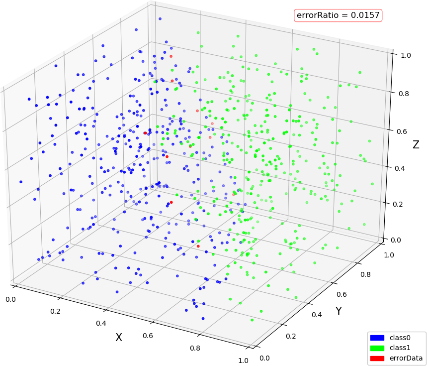
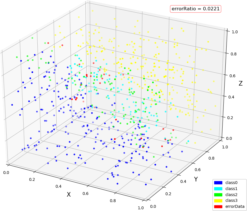
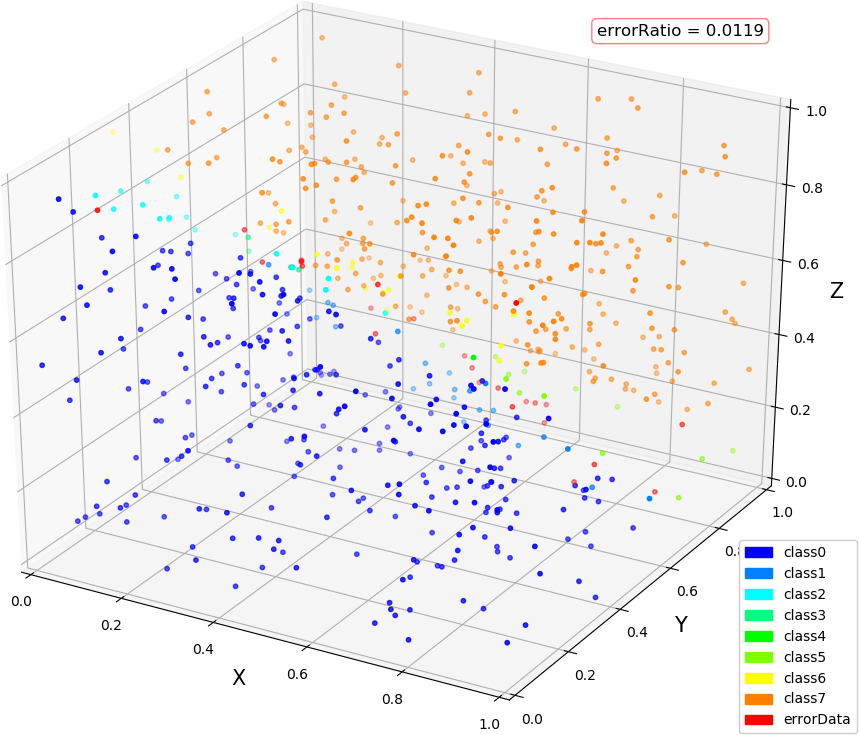
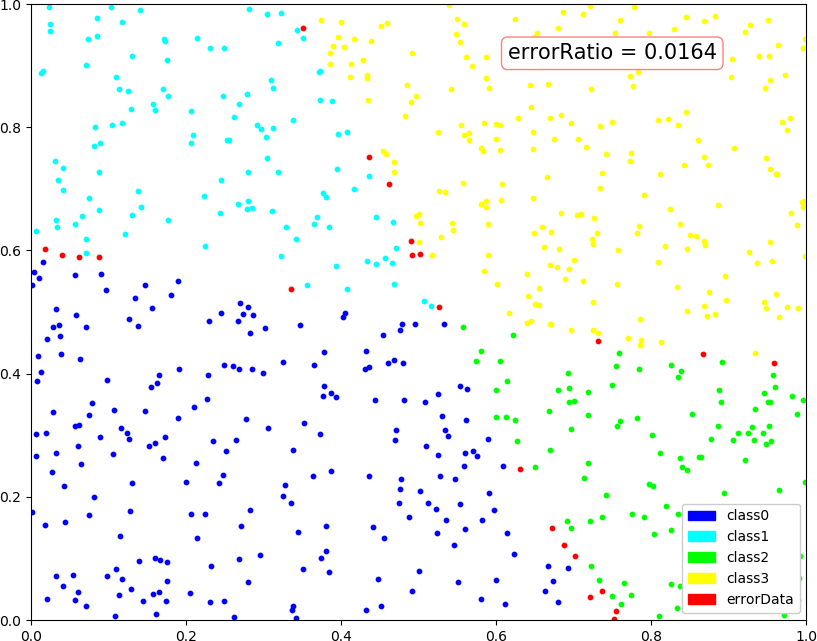
● 输出结果,写明了输入维度,中间层维度,输出维度,前三个的训练论轮较多,偷懒打表了。可见数据维度越高训练时间越长,单纯增加或减少中间层的神经元个数不一定会改善精度或训练速度
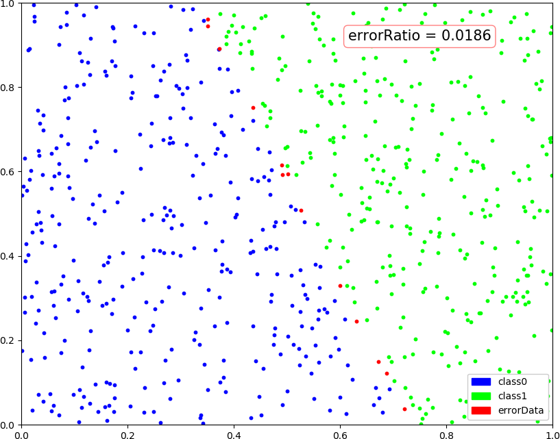
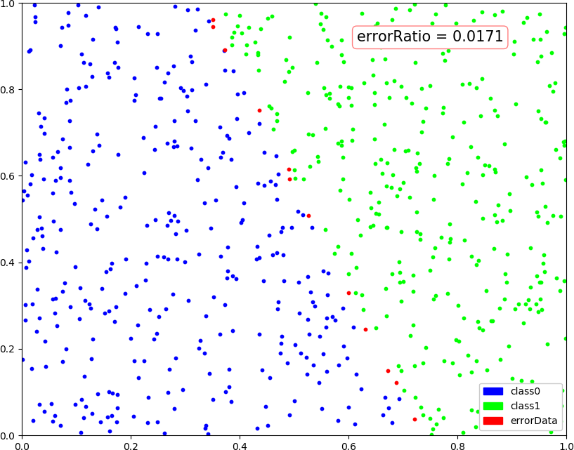
count =  1 , error =  0.009960528091961436
dimIn = 3, dimMid = 4, dimOut = 1, errorRatio = 0.0157

count =  1 , error =  0.009961970578632297
dimIn = 3, dimMid = 4, dimOut = 2, errorRatio = 0.0221

count =  500 , error =  0.01439582086937022
dimIn = 3, dimMid = 4, dimOut = 3, errorRatio = 0.0119

count =  185 , error =  0.01000959424865353
count =  186 , error =  0.009996998960686504
dimIn = 2, dimMid = 4, dimOut = 1, errorRatio = 0.0171

count =  368 , error =  0.010011781526423453
count =  369 , error =  0.009995998845193808
dimIn = 2, dimMid = 4, dimOut = 2, errorRatio = 0.0164

count =  183 , error =  0.01000216394730506
count =  184 , error =  0.009989705432858783
dimIn = 2, dimMid = 3, dimOut = 1, errorRatio = 0.0186

count =  188 , error =  0.010007727220216402
count =  189 , error =  0.009995233860763614
dimIn = 2, dimMid = 5, dimOut = 1, errorRatio = 0.0171
● 画图:(3,4,1),(3,4,2),(3,4,3)
● 画图:(2,4,1),(2,4,2),(2,3,1),(2,5,1)

● 画图:(1,3,1)
