Conventional AM Demodulation
The conventional AM is inferior to DSB-AM and SSB-AM when
power and SNR are considered. The reason is that a usually large part of the modulated
signal power is in the carrier component that does not carry information. The role of
the carrier component is to make the demodulation of the conventional AM easier via
envelope detection, as opposed to coherent demodulation required for DSB-AM and
SSB-AM. Therefore, demodulation of AM signals is significantly less complex than
the demodulation of DSB-AM and SSB-AM signals. Hence, this modulation scheme is
widely used in broadcasting, where there is a single transmitter and numerous receivers
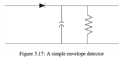
whose cost should be kept low. In envelope detection the envelope of the modulated
signal is detected via a simple circuit consisting of a diode, a resistor, and a capacitor,
as shown in Figure.
Matlab Coding
1 % MATLAB script for Illustrative Problem 3.9. 2 % Demonstration script for envelope detection. The message signal 3 % is +1 for 0 < t < t0/3, -2 for t0/3 < t < 2t0/3, and zero otherwise. 4 echo on 5 t0=.15; % signal duration 6 ts=0.001; % sampling interval 7 fc=250; % carrier frequency 8 a=0.85; % modulation index 9 fs=1/ts; % sampling frequency 10 t=[0:ts:t0]; % time vector 11 df=0.25; % required frequency resolution 12 % message signal 13 m=[ones(1,t0/(3*ts)),-2*ones(1,t0/(3*ts)),zeros(1,t0/(3*ts)+1)]; 14 c=cos(2*pi*fc.*t); % carrier signal 15 m_n=m/max(abs(m)); % normalized message signal 16 [M,m,df1]=fftseq(m,ts,df); % Fourier transform 17 f=[0:df1:df1*(length(m)-1)]-fs/2; % frequency vector 18 u=(1+a*m_n).*c; % modulated signal 19 [U,u,df1]=fftseq(u,ts,df); % Fourier transform 20 env=env_phas(u); % Find the envelope. 21 dem1=2*(env-1)/a; % Remove dc and rescale. 22 signal_power=spower(u(1:length(t))); % power in modulated signal 23 noise_power=signal_power/100; % noise power 24 noise_std=sqrt(noise_power); % noise standard deviation 25 noise=noise_std*randn(1,length(u)); % Generate noise. 26 r=u+noise; % Add noise to the modulated signal. 27 [R,r,df1]=fftseq(r,ts,df); % Fourier transform 28 env_r=env_phas(r); % envelope, when noise is present 29 dem2=2*(env_r-1)/a; % Demodulate in the presence of noise.
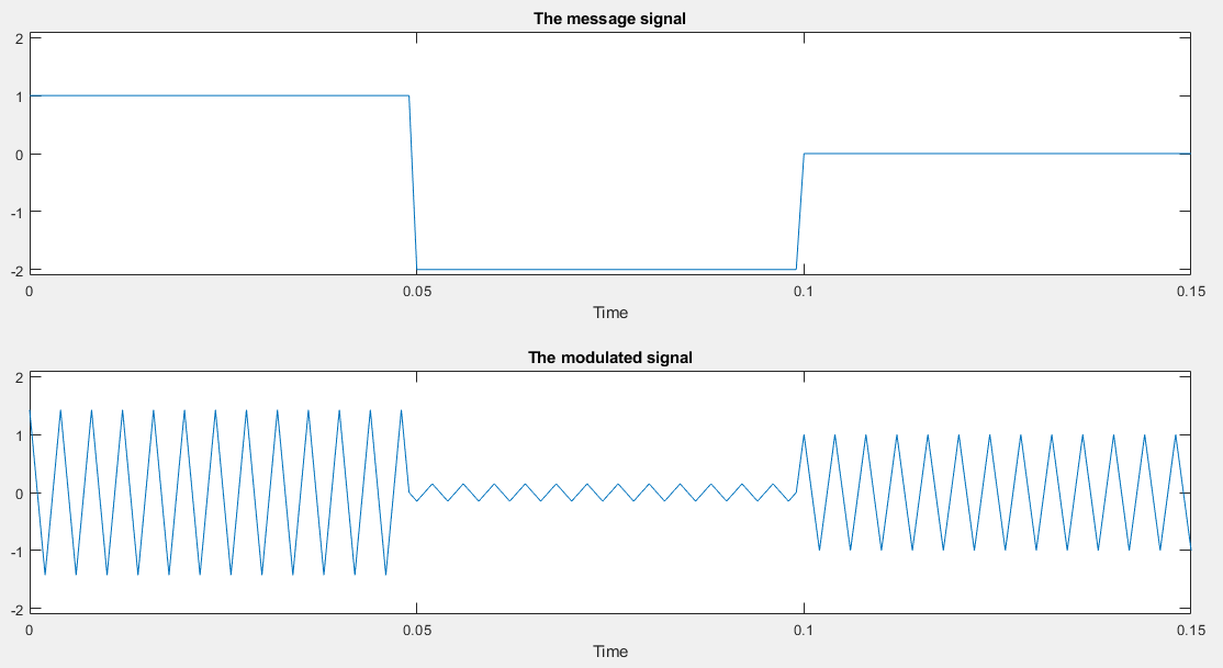
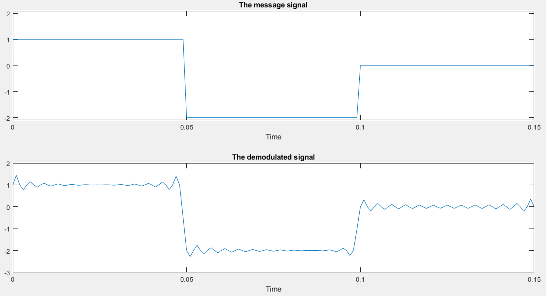
30 pause % Press any key to see a plot of the message. 31 subplot(2,1,1) 32 plot(t,m(1:length(t))) 33 axis([0 0.15 -2.1 2.1]) 34 xlabel('Time') 35 title('The message signal') 36 pause % Press any key to see a plot of the modulated signal. 37 subplot(2,1,2) 38 plot(t,u(1:length(t))) 39 axis([0 0.15 -2.1 2.1]) 40 xlabel('Time') 41 title('The modulated signal') 42 pause % Press a key to see the envelope of the modulated signal. 43 clf 44 subplot(2,1,1) 45 plot(t,u(1:length(t))) 46 axis([0 0.15 -2.1 2.1]) 47 xlabel('Time') 48 title('The modulated signal') 49 subplot(2,1,2) 50 plot(t,env(1:length(t))) 51 xlabel('Time') 52 title('Envelope of the modulated signal') 53 pause % Press a key to compare the message and the demodulated signal. 54 clf 55 subplot(2,1,1) 56 plot(t,m(1:length(t))) 57 axis([0 0.15 -2.1 2.1]) 58 xlabel('Time') 59 title('The message signal') 60 subplot(2,1,2) 61 plot(t,dem1(1:length(t))) 62 xlabel('Time') 63 title('The demodulated signal') 64 pause % Press a key to compare in the presence of noise. 65 clf 66 subplot(2,1,1) 67 plot(t,m(1:length(t))) 68 axis([0 0.15 -2.1 2.1]) 69 xlabel('Time') 70 title('The message signal') 71 subplot(2,1,2) 72 plot(t,dem2(1:length(t))) 73 xlabel('Time') 74 title('The demodulated signal in the presence of noise')
The message and the envelope of the modulated signal
The envelope of the modulated signal

Compare the message and the demodulated signal
compare message and the demodulated signal in the presence of noise

Reference,
1. <<Contemporary Communication System using MATLAB>> - John G. Proakis