使用R语言预测产品销量

使用R语言预测产品销量

通过不同的广告投入，预测产品的销量。因为响应变量销量是一个连续的值，所以这个问题是一个回归问题。数据集共有200个观测值，每一组观测值对应一种市场情况。

数据特征

• TV：对于一个给定市场的单一产品，用于电视上的广告费用（以千为单位）
• Radio：用于广告媒体上投资的广告费用
• Newspaper：用于报纸媒体上的广告费用

响应

• Sales：对应产品的销量

加载数据

> data <- read.csv("http://www-bcf.usc.edu/~gareth/ISL/Advertising.csv",colClasses=c("NULL",NA,NA,NA,NA))
> head(data)     
  TV Radio Newspaper Sales
1 230.1  37.8      69.2  22.1
2  44.5  39.3      45.1  10.4
3  17.2  45.9      69.3   9.3
4 151.5  41.3      58.5  18.5
5 180.8  10.8      58.4  12.9
6   8.7  48.9      75.0   7.2
# 显示Sales和TV的关系
> plot(data$TV, data$Sales, col="red", xlab='TV', ylab='sales')

# 用线性回归拟合Sales和TV广告的关系
> fit=lm(Sales~TV,data=data)
# 查看估算出来的系数
> coef(fit)
(Intercept)          TV 
 7.03259355  0.04753664
# 显示拟合出来的模型的线
> abline(fit)

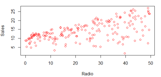
# 显示Sales和Radio的关系
> plot(data$Radio, data$Sales, col="red", xlab='Radio', ylab='Sales')

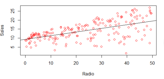
# 用线性回归拟合Sales和Radio广告的关系
> fit1=lm(Sales~Radio,data=data)
# 查看估算出来的系数
> coef(fit1)
(Intercept)       Radio 
  9.3116381   0.2024958
# 显示拟合出来的模型的线
> abline(fit1)

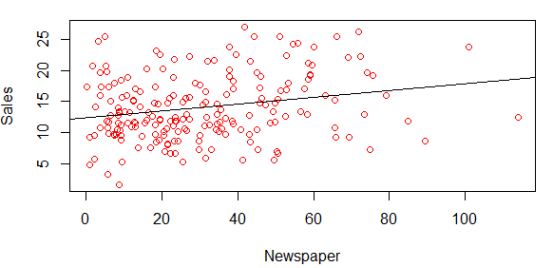
# 显示Sales和Newspaper的关系
> plot(data$Newspaper, data$Sales, col="red", xlab='Radio', ylab='Sales')

# 用线性回归拟合Sales和Radio广告的关系
> fit2=lm(Sales~Newspaper,data=data)
# 查看估算出来的系数
> coef(fit2)
(Intercept)   Newspaper 
 12.3514071   0.0546931
# 显示拟合出来的模型的线
> abline(fit2)

# 创建散点图矩阵
> pairs(~Sales+TV+Radio+Newspaper,data=data, main="Scatterplot Matrix")

第一行图形显示TV，Radio，Newspaper对Sales的影响。纵轴为Sales，横轴分别为TV，Radio，Newspaper。从图中可以看出，TV特征和销量是有比较强的线性关系的。

划分训练集和测试集

> trainRowCount <- floor(0.8 * nrow(data))
> set.seed(1)
> trainIndex <- sample(1:nrow(data), trainRowCount)
> train <- data[trainIndex,]
> test <- data[-trainIndex,]
> dim(data)
[1] 200   4
> dim(train)
[1] 160   4
> dim(test)
[1] 40  4

拟合线性回归模型

> model <- lm(Sales~TV+Radio+Newspaper, data=train)
> summary(model)
Call:
lm(formula = Sales ~ TV + Radio + Newspaper, data = train)

Residuals:
    Min      1Q  Median      3Q     Max 
-8.7734 -0.9290  0.2475  1.2213  2.8971 

Coefficients:
             Estimate Std. Error t value Pr(>|t|)    
(Intercept)  2.840243   0.353175   8.042 2.07e-13 ***
TV           0.046178   0.001579  29.248  < 2e-16 ***
Radio        0.189668   0.009582  19.795  < 2e-16 ***
Newspaper   -0.001156   0.006587  -0.176    0.861    
---
Signif. codes:  0 ‘***’ 0.001 ‘**’ 0.01 ‘*’ 0.05 ‘.’ 0.1 ‘ ’ 1

Residual standard error: 1.745 on 156 degrees of freedom
Multiple R-squared:  0.8983,    Adjusted R-squared:  0.8963 
F-statistic: 459.2 on 3 and 156 DF,  p-value: < 2.2e-16

预测和计算均方根误差

> predictions <- predict(model, test)
> mean((test["Sales"] - predictions)^2)
[1] 2.050666

特征选择

在之前的各变量和销量之间关系中，我们看到Newspaper和销量之间的线性关系比较弱，并且上面模型中Newspaper的系数为负数，现在去掉这个特征，看看线性回归预测的结果的均方根误差。

 

> model1 <- lm(Sales~TV+Radio, data=train)
> summary(model1)
Call:
lm(formula = Sales ~ TV + Radio, data = train)

Residuals:
    Min      1Q  Median      3Q     Max 
-8.7434 -0.9121  0.2538  1.1900  2.9009 

Coefficients:
            Estimate Std. Error t value Pr(>|t|)    
(Intercept) 2.821417   0.335455   8.411 2.35e-14 ***
TV          0.046157   0.001569  29.412  < 2e-16 ***
Radio       0.189132   0.009053  20.891  < 2e-16 ***
---
Signif. codes:  0 ‘***’ 0.001 ‘**’ 0.01 ‘*’ 0.05 ‘.’ 0.1 ‘ ’ 1

Residual standard error: 1.74 on 157 degrees of freedom
Multiple R-squared:  0.8983,    Adjusted R-squared:  0.897 
F-statistic:   693 on 2 and 157 DF,  p-value: < 2.2e-16

> predictions1 <- predict(model1, test)
> mean((test["Sales"] - predictions1)^2)
[1] 2.050226

 

从上可以看到2.050226<2.050666，将Newspaper这个特征移除后，得到的均方根误差变小了，说明Newspaper不适合作为预测销量的特征，则去掉Newspaper特征后得到了新的模型。