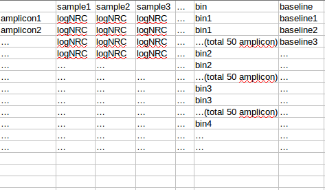
进行数据初步处理(perl)
- 统计amplicon的RC(read counts),并且相互overlap大于75%的amplicon合并起来
- 统计每个amplicon的GC含量,均值,

性别识别并校正,文库大小、长度、GC含量标准化
-
文库大小标准化
某个sample的文库大小(read counts * amplicon length) / 平均每个ampicon文库大小(sum(read counts * amplicon length) / amplicon size))
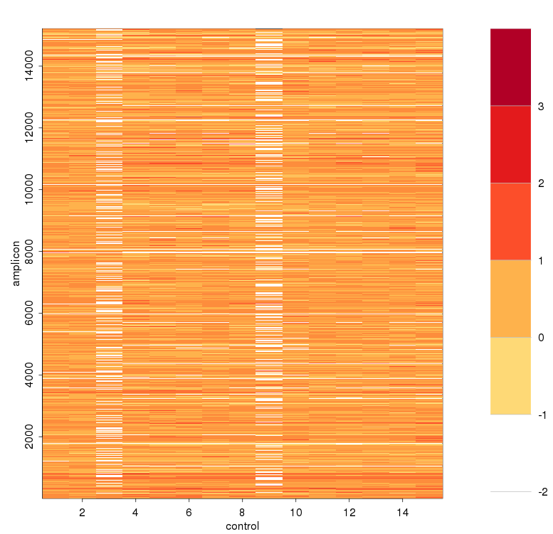
标准化前
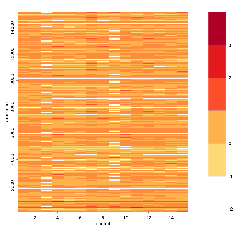
标准化后
-
性别识别并校正
使用mcluster基于高斯混合模型对X染色体NRC与平均X染色体NRC比例值进行聚类,如果聚成两类,猜测混合的男女数据,如果一类,猜测全是男或者全是女,需要对男样本的X染色体NRC*2
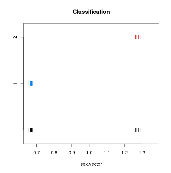
可见混合了男女sample -
去除GC < 0.1 分位数和 GC > 0.9 分位数的amplicon,不进行loess
-
去除length < 0.005 分位数和 length > 0.995 分位数的amplicon,不进行loess
-
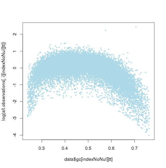
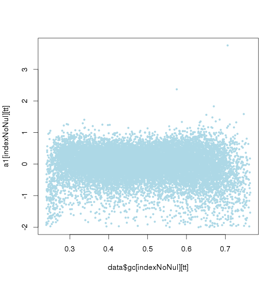
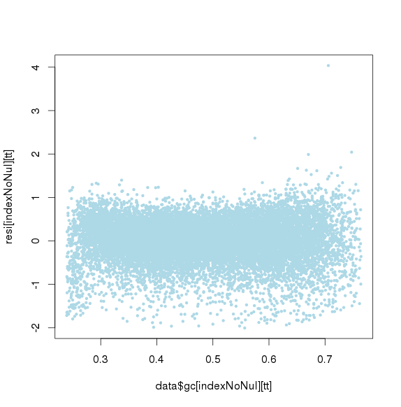
使用loess进行长度、GC标准化(标准化时使用log NRC)
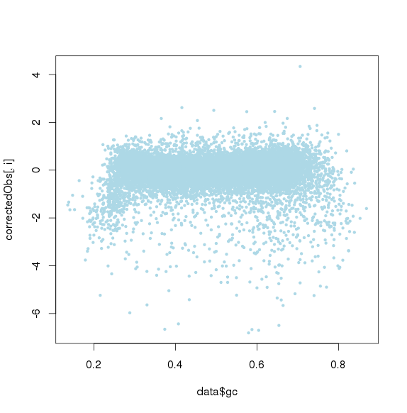
GC标准化前
GC标准化后
GC再次标准化后(去除第一次标准化后小于或大于threthold的amplicon)
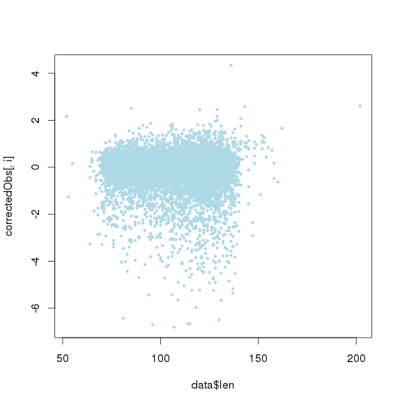
GC标准化后,长度标准化前
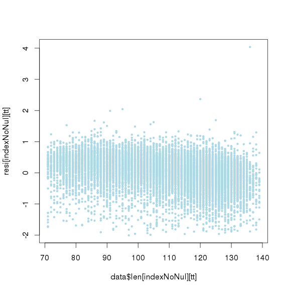
长度标准化后
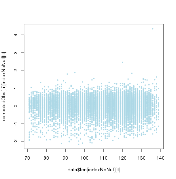
包括GC和amplicon length 极端值时的点图
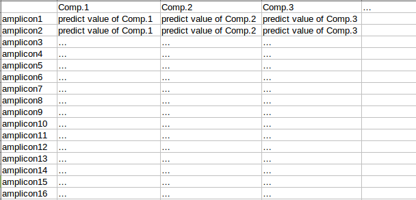
进行ICA(独立成分分析)
- 去除深度远远低于其他样品的amplicon,这种个别sample中amplicon的变化并不是实验偏差造成的
每两两样品间作线性回归,计算预测值,如果实际值比预测值低2NRC,那么在ICA中不考虑该amplicon - ICA
使用fastICA进行独立成分分析,G函数选择logcosh,这些独立成分(或者主成分)认为是主要的实验偏差。
各主成分解释变异的比例(使用主成分函数princomp计算,fastICA中没有显示)
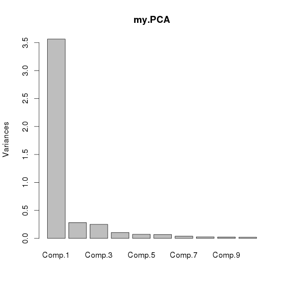
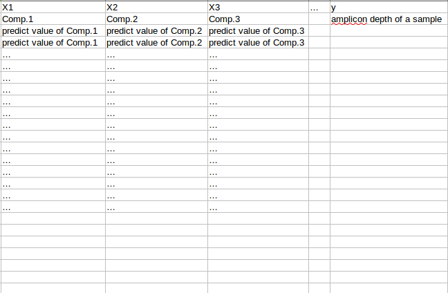
所以只取一个主成分,计算各个主成分与amplicon在所有样品中平均logNRC的相关系数,取最大的一个主成分作为主成分, - 按照amplicon 平均深度标准化,并* K权重(ICA的结果中有)得到每个amplicon在各个主成分的值,得到一个行为amplicon,列为PCA的矩阵
- 每个amplicon根据sample depth 进行校正后的logNRC(减去sample mean depth)*主要主成分的载荷(比如PC1的载荷)求均值,得到每个amplicon的baseline
进行ICA之前的logNRC
计算baseline时sample之间校正,减去sample 平均深度之后
可见对部分amplicon进行了一些校正,特别是平均深度教少的两个amplicon - 取baseline > -2的amplicon出来,logNRC与主成分值进行线性回归,求残差,得到去除实验偏差造成的影响,对这些点进行方差校正
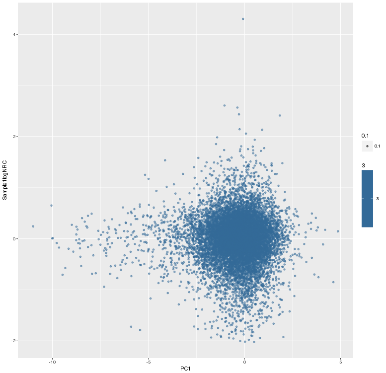
主成分标准化前,logNRC Vs PC1

主成分标准化后,logNRC Vs PC1
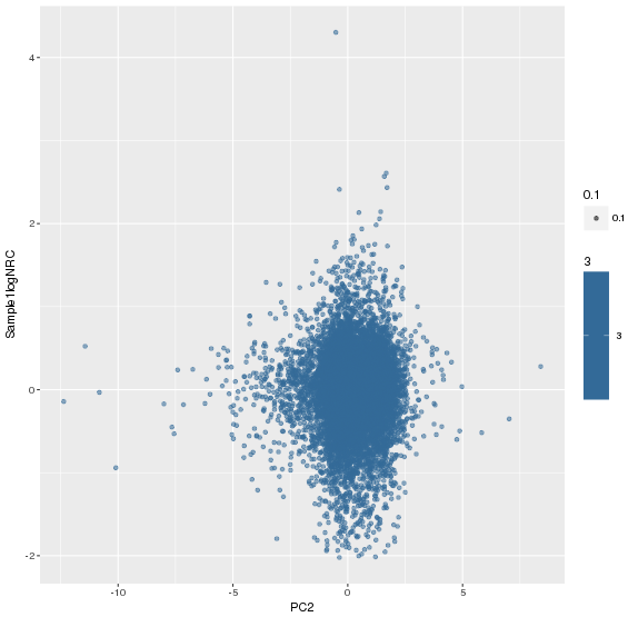
主成分标准化前,logNRC Vs PC2

主成分标准化后,logNRC Vs PC2
线性回归的系数非常小,所以影响不大
Coefficients:
            Value   Std. Error t value
(Intercept)  0.0287  0.0050     5.7175
S[tt, ]1     0.0054  0.0031     1.7508
S[tt, ]2    -0.0076  0.0041    -1.8356
S[tt, ]3    -0.0018  0.0040    -0.4615
S[tt, ]4    -0.0023  0.0028    -0.8080
S[tt, ]5    -0.0016  0.0021    -0.7327
S[tt, ]6    -0.0012  0.0027    -0.4470
S[tt, ]7     0.0000  0.0024     0.0087
S[tt, ]8    -0.0020  0.0018    -1.1415
S[tt, ]9    -0.0012  0.0021    -0.5675
S[tt, ]10   -0.0008  0.0016    -0.4773
S[tt, ]11   -0.0022  0.0018    -1.2418
S[tt, ]12    0.0010  0.0016     0.6654
S[tt, ]13   -0.0014  0.0018    -0.7660
S[tt, ]14   -0.0015  0.0013    -1.1455
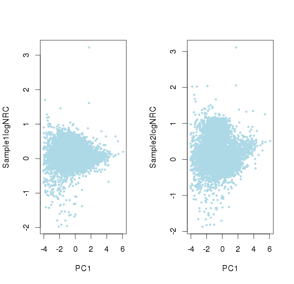
并且可以看出logNRC方差随着PC1(logNRC)增大而减少
方差校正
不同样本总的方差可以看出不同,有的样本更加离散
-
认为最后的logNRC服从正态分布,均值是0,而方差可以由(PC1解释)
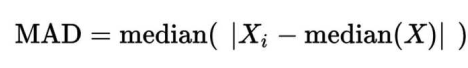
取logNRC > -2的amplicon,求出所有logNRC的绝对中位差(MAD),sd.all,再求出每个sample绝对中位差sd.sample,最后每个sample中,logNRC进行方差校正logNRC = (logNRC - median(logNRC))/(sd.sample/sd.all) + median(logNRC)
校正后
-
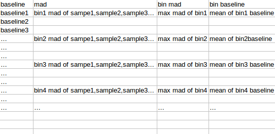
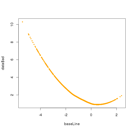
将observation 的amplicon 按照baseline从小到达排序,分成每50个amplicon 分一个bin,对bin内的每个sample的50个amplicon的logNRC求组内mad(旧版本是sd),将该bin的mad设置为多个sample中最大的mad(最大组内mad),该bin的平均baseline作为该bin 的baseline
-
对bin mad和bin baseline用loess作线性回归,得到loess模型,将所有amplicon baseline输入,得到amplicon mad 的预测值,再求出每个sample 的amplicon logNRC的mad值,将该预测值/最大sample mad值,得到的比值作为该amplicon的sd

library(mclust) #for clustering to detect gender of control samples
library(MASS)
library(scales) #for graph transparency
library(fastICA) #for ICA
library(psych)
library(ggplot2)
inputFile <-"~/project/ONCOCNV_RES/Control.stats.txt"
controlFile <- "~/project/ONCOCNV_RES/MyControl.stats.Processed.txt"
GCfile <- "~/project/ONCOCNV_RES/target.GC.txt"
NUMBEROFPC=3
minFractionOfShortOrLongAmplicons=0.05 #change if needed
NUMBEROFPC=3
if (NUMBEROFPC<1) {
NUMBEROFPC=3
}
if (NUMBEROFPC>3) {
cat("Can keep maximum 3 principal components")
NUMBEROFPC=3
}
magicThreshold=-2 #normalized read count less than this value will not be considered if it is not consistent between the control replicates
maxLoess=50000 #maximum number of points for the regression, starting from v6.5
dataTable <-read.table(inputFile, header=TRUE);
data<-data.frame(dataTable)
ncont <- length(data)-6
all.observations <- data[,7:length(data)]
data$len<-data$end-data$start
#pairs.panels(all.observations[,c(1:5)])
if (ncont >1) {
totalTargetLen<-sum(all.observations[,1]*data$len)
}else {
totalTargetLen<-sum(all.observations*data$len)
}
nulInd <- NULL
if (ncont >1) {
for (i in (1:(ncont))) {
nulInd<-c(nulInd,which(all.observations[,i]==0 | is.na(all.observations[,i])==TRUE | data$chr=="chrX"| data$chr=="chrY"| data$chr=="X"| data$chr=="Y") )
all.observations[,i]<- all.observations[,i]*data$len/totalTargetLen*length(data$len) #for ampli-based, correct back for amplicon length
}
noNulIdex <-c(1:length(all.observations[,1]))
}else {
nulInd<-c(nulInd,which(all.observations==0 | is.na(all.observations)==TRUE | data$chr=="chrX"| data$chr=="chrY" | data$chr=="X"| data$chr=="Y") )
all.observations<- all.observations*data$len/totalTargetLen*length(data$len) #for ampli-based, correct back for amplicon length
noNulIdex <-c(1:length(all.observations))
}
#pairs.panels(all.observations[,c(1:5)])
if (length(nulInd)>0) {
indexNoNul<- noNulIdex[-sort(unique(nulInd))]
} else {
indexNoNul<- noNulIdex
}
if (ncont >1) {
observations <- all.observations[indexNoNul,]
} else {
observations <- all.observations[indexNoNul]
}
noMakeNA<-NULL
if (ncont >1){
NUMBEROFPC = ncont-1;
#detect female/male: starting from version 5.0:
sex.vector=NULL
tt <- which(all.observations[,i]>0 & is.na(all.observations[,i])==FALSE & (data$chr=="chrX" | data$chr=="X"))
if (length(tt)>0) {
for (i in (1:ncont)) {
sex.vector[i] <- sum(all.observations[,i][tt] )/ sum(all.observations[tt,] )*ncont
}
mc <- Mclust(sex.vector,G=c(1,2))
#plot(mc)
if (mc$G==2) {
cat ("Warning: you have both male and female samples in the control. We will try to assign sex using read coverage on chrX
")
sex.vector <- mc$classification/2
cat (sex.vector);cat("
")
}else {
cat ("all your samples have the same number of chrX. We assume they are all male; change the code for assume they are all female
")
propX = sum(all.observations[tt,])/length(tt)/sum(all.observations[-tt,])*length(all.observations[-tt,1])
for (i in (1:ncont)) {
if (propX<0.9) {sex.vector[i] <- 0.5;} else {sex.vector[i] <- 1;}
#sex.vector[i] <- 1 #uncomment if all your control samples are female
}
}
#correct the number of reads on chr X for Gender #starting from version 5.0:
for (i in (1:ncont)) {
tt <- which(all.observations[,i]>0 & is.na(all.observations[,i])==FALSE & (data$chr=="chrX" | data$chr=="chrY" | data$chr=="X" | data$chr=="Y"))
all.observations[,i][tt]<- all.observations[,i][tt] / sex.vector[i]
}
}
lmin<-quantile(data$len,probs =0.005, na.rm = TRUE)
lmax<-quantile(data$len,probs = 0.995, na.rm = TRUE)
minFrac = length(which(data$len<lmin))/length(data$len) #strictly from v6.5
maxFrac = length(which(data$len>lmax))/length(data$len)
#remove too short or too long amplicons (only if there are less than 5% of them: parameter minFractionOfShortOrLongAmplicons)
if (minFrac< minFractionOfShortOrLongAmplicons &maxFrac<minFractionOfShortOrLongAmplicons) {
nulInd <- which(data$len<lmin | data$len>lmax)
} else if (minFrac< minFractionOfShortOrLongAmplicons &maxFrac>=minFractionOfShortOrLongAmplicons) {
nulInd <- unique(which(data$len<lmin ))
} else if (minFrac>= minFractionOfShortOrLongAmplicons &maxFrac<minFractionOfShortOrLongAmplicons) {
nulInd <- unique(which( data$len>lmax))
}
Control.stats.GC <- read.delim(GCfile)
data$gc<-Control.stats.GC$GC
lmin<-quantile(data$gc,probs =0.01, na.rm = TRUE)
lmax<-quantile(data$gc,probs = 0.99, na.rm = TRUE)
nulInd <- unique(c(nulInd,which(data$gc<=lmin | data$gc>=lmax)))
data$mean <-rowMeans(all.observations)
lmin<-quantile(data$mean,probs =0.01, na.rm = TRUE)
lmax<-quantile(data$mean,probs = 0.99, na.rm = TRUE)
minFrac = length(which(data$mean<=lmin))/length(data$mean)
maxFrac = length(which(data$mean>=lmax))/length(data$mean)
#remove too short or too long amplicons (only if there are less than 5% of them: parameter minFractionOfShortOrLongAmplicons)
if (minFrac< minFractionOfShortOrLongAmplicons &maxFrac<minFractionOfShortOrLongAmplicons) {
nulInd <- unique(c(nulInd,which(data$mean<=lmin | data$mean>=lmax)))
} else if (minFrac< minFractionOfShortOrLongAmplicons &maxFrac>=minFractionOfShortOrLongAmplicons) {
nulInd <- unique(c(nulInd,which(data$mean<=lmin )))
} else if (minFrac>= minFractionOfShortOrLongAmplicons &maxFrac<minFractionOfShortOrLongAmplicons) {
nulInd <- unique(c(nulInd,which( data$mean>=lmax)))
}
noNulIdex <-c(1:length(all.observations[,1]))
indexNoNul<- noNulIdex[-sort(unique(nulInd))]
observations <- all.observations[indexNoNul,]
correctedObs=matrix(nrow=length(all.observations[,1]),ncol=length(all.observations),byrow=T)
for (i in (1:(ncont))) {
# tt <- which(all.observations[,i][indexNoNul]>0 & log(all.observations[,i][indexNoNul])>magicThreshold)
# gcCount.spl <- smooth.spline(data$gc[indexNoNul][tt], log(all.observations[,i][indexNoNul][tt]))
# predictions <- predict(gcCount.spl,data$gc)$y
# a1 <- log(all.observations[,i])-predictions
#
# #recorrect the at the tails of GC-content #need it because of the strange cases like control 3 and 9...
# tt <- which(all.observations[,i][indexNoNul]>0 & a1[indexNoNul] > magicThreshold)
# gcCount.spl <- smooth.spline(data$gc[indexNoNul][tt], a1[indexNoNul][tt])
# predictions <- predict(gcCount.spl,data$gc)$y
# resi <- a1-predictions
# len.spl <- smooth.spline(data$len[indexNoNul][tt], resi[indexNoNul][tt])
# correctedObs[,i] <- resi-predict(len.spl,data$len)$y
# correctedObs[,i][-indexNoNul] <- NA
tt <- which(all.observations[,i][indexNoNul]>0 & log(all.observations[,i][indexNoNul])>magicThreshold) #starting from 5.3 - LOESS
if (length(tt)>maxLoess) {tt=sort(sample(tt, maxLoess, replace = FALSE))} #starting from v6.5 to use on exome data
#plot(data$gc[indexNoNul][tt],log(all.observations[,i][indexNoNul][tt]),cex=0.5,pch=19,col="lightblue")
gcCount.loess <- loess(log(all.observations[,i][indexNoNul][tt])~data$gc[indexNoNul][tt], control = loess.control(surface = "direct"),degree=2) #loess starting from version 5.2
predictions1<- predict (gcCount.loess,data$gc)
a1 <- log(all.observations[,i])-predictions1
#plot(data$gc[indexNoNul][tt],a1[indexNoNul][tt],cex=0.5,pch=19,col="lightblue")
tt <- which(all.observations[,i][indexNoNul]>0 & a1[indexNoNul] > magicThreshold)
if (length(tt)>maxLoess) {tt=sample(tt, maxLoess, replace = FALSE)} #starting from v6.5 to use on exome data
#plot(data$gc[indexNoNul][tt],a1[indexNoNul][tt],cex=0.5,pch=19,col="lightblue")
gcCount.loess <- loess(a1[indexNoNul][tt]~data$gc[indexNoNul][tt],control = loess.control(surface = "direct"),degree=2) #loess starting from version 5.2
predictions<- predict (gcCount.loess,data$gc)
resi <- a1-predictions
#plot(data$gc[indexNoNul][tt],resi[indexNoNul][tt],cex=0.5,pch=19,col="lightblue")
#plot(data$len[indexNoNul][tt],resi[indexNoNul][tt],cex=0.5,pch=19,col="lightblue")
len.loess <- loess( resi[indexNoNul][tt]~data$len[indexNoNul][tt], control = loess.control(surface = "direct"),degree=2)
correctedObs[,i] <- resi-predict(len.loess,data$len)
#plot(data$len[indexNoNul][tt],correctedObs[,i][indexNoNul][tt],cex=0.5,pch=19,col="lightblue")
#plot(data$gc[indexNoNul][tt],correctedObs[,i][indexNoNul][tt],cex=0.5,pch=19,col="lightblue")
#plot(data$len,correctedObs[,i],cex=0.5,pch=19,col="lightblue")
#plot(data$gc,correctedObs[,i],cex=0.5,pch=19,col="lightblue")
}
for (i in (1:(ncont))) {
correctedObs[,i][-indexNoNul] <- NA
correctedObs[,i][which(is.infinite(correctedObs[,i]))] <- NA
#plot(data$len,correctedObs[,i],col=2)
}
observations <- correctedObs[indexNoNul,] #they are already in LOG scale!!!
makeNA <- NULL
for (i in (1:ncont)) {
for (j in (1:ncont)) {
if (i!=j) {
my.lm <- rlm((observations[,j]) ~(observations[,i]))
#hist((observations[,j])-my.lm$fitted,n=100)
predictions <- (correctedObs[,i])*my.lm$coefficients[2]+my.lm$coefficients[1]
tt <- (which ((correctedObs[,j])-predictions<magicThreshold))
tt2 <- which(is.na(correctedObs[,j]))
makeNA<-unique(c(makeNA,tt,tt2))
}
}
}
if(length(makeNA)>0) {
noNulIdex <-c(1:length(correctedObs[,1]))
indexToFit<- noNulIdex[-sort(unique(makeNA))]
indexToFit<- intersect(indexToFit,indexNoNul)
} else {
indexToFit<- indexNoNul
}
observations <- correctedObs[indexToFit,]
#do ICA1 to for remaining points:
X<-observations #observations are in LOG scale
a <- fastICA(X,NUMBEROFPC, alg.typ = "parallel", fun = "logcosh", alpha = 1,
method = "C", row.norm = FALSE, maxit = 200,
tol = 0.000001, verbose = TRUE)
my.PCA <- princomp(X)
cumExplainVar<- cumsum(my.PCA[["sdev"]]^2)/sum(my.PCA[["sdev"]]^2)
cat("Explained variance by the first pronicpal components of PCA:")
cat(names(cumExplainVar))
cat (cumExplainVar)
#screeplot(my.PCA)
mainComp=1;myCor=0;
for (i in (1:NUMBEROFPC)) {
if(abs(cor(rowMeans(X),(a$X %*% a$K)[,i]))>myCor) {
myCor=abs(cor(rowMeans(X),a$X %*% a$K[,i]));
mainComp=i;
}
}
if (cor(rowMeans(X),a$X %*% a$K[,mainComp])<0) {a$K=-a$K;}
shifts<-colMeans(X)
controlFilePDF<-paste(controlFile,".pdf",sep="")
pdf(file = controlFilePDF, width=7*ncont/3, height=7*ncont/3)
par(mfrow=c((ncont-1),(ncont-1)))
atmp<-NULL
CellCounter=1
for (i in (1:(ncont-1))) {
for (j in (1:(ncont-1))) {
if (i<=j) {atmp<-c(atmp,CellCounter);CellCounter=CellCounter+1} else {atmp<-c(atmp,0);}
}
}
layout(matrix(c(atmp), ncont-1, ncont-1, byrow = TRUE))
for (i in (1:(ncont-1))) {
for (j in ((i+1):ncont)) {
my.lm <- rlm((observations[,j]) ~(observations[,i]))
myCstr1 <- paste("control",i)
myCstr2 <- paste("control",j)
plot((observations[,i]),(observations[,j]),xlab=bquote(~NRC[.(myCstr1)] ),ylab=bquote(~NRC[.(myCstr2)] ),
col="white",pch=21,cex=0.8) #553
points((correctedObs[,i])[makeNA],(correctedObs[,j])[makeNA],
col="darkgrey",bg=alpha("grey",0.5),pch=21,cex=0.8)
tt<-which((observations[,i])<(observations[,j]))
points((observations[,i])[tt],(observations[,j])[tt],
col=colors()[553],bg=alpha(colors()[553],0.5),pch=21,cex=0.8)
points((observations[,i])[-tt],(observations[,j])[-tt],
col=colors()[90],bg=alpha(colors()[90],0.5),pch=21,cex=0.8)
abline(my.lm,col="grey",lwd=2)
abline(a=0,b=1,col="black",lwd=2,lty=3)
}
}
dev.off()
} else {
NUMBEROFPC = 1;
#detect female/male: starting from version 5.0:
tt <- which(all.observations>0 & is.na(all.observations)==FALSE & (data$chr=="chrX" | data$chr=="X"))
tt2 <- which(all.observations>0 & is.na(all.observations)==FALSE & (data$chr!="chrX"| data$chr=="X"))
if (length(tt)>0) {
propX = sum(all.observations[tt])/length(tt)/(sum(all.observations[tt2])/length(tt2))
if (propX<0.9) {sex.vector <- 0.5;} else {sex.vector <- 1;}
#correct the number of reads on chr X for Gender #starting from version 5.0:
tt <- which(all.observations>0 & is.na(all.observations)==FALSE & (data$chr=="chrX" | data$chr=="chrY" | data$chr=="X" | data$chr=="Y"))
all.observations[tt]<- all.observations[tt] / sex.vector
}
lmin<-quantile(data$len,probs =0.005, na.rm = TRUE)
lmax<-quantile(data$len,probs = 0.995, na.rm = TRUE)
minFrac = length(which(data$len<lmin))/length(data$len) #strictly from v6.5
maxFrac = length(which(data$len>lmax))/length(data$len)
#remove too short or too long amplicons (only if there are less than 5% of them: parameter minFractionOfShortOrLongAmplicons)
if (minFrac< minFractionOfShortOrLongAmplicons &maxFrac<minFractionOfShortOrLongAmplicons) {
nulInd <- which(data$len<lmin | data$len>lmax)
} else if (minFrac< minFractionOfShortOrLongAmplicons &maxFrac>=minFractionOfShortOrLongAmplicons) {
nulInd <- unique(which(data$len<lmin ))
} else if (minFrac>= minFractionOfShortOrLongAmplicons &maxFrac<minFractionOfShortOrLongAmplicons) {
nulInd <- unique(which( data$len>lmax))
}
Control.stats.GC <- read.delim(GCfile)
data$gc<-Control.stats.GC$GC
lmin<-quantile(data$gc,probs =0.01, na.rm = TRUE)
lmax<-quantile(data$gc,probs = 0.99, na.rm = TRUE)
nulInd <- unique(c(nulInd,which(data$gc<=lmin | data$gc>=lmax)))
data$mean <-all.observations
lmin<-quantile(data$mean,probs =0.01, na.rm = TRUE)
lmax<-quantile(data$mean,probs = 0.99, na.rm = TRUE)
nulInd <- unique(c(nulInd,which(data$mean<=lmin | data$mean>=lmax)))
noNulIdex <-c(1:length(all.observations))
indexNoNul<- noNulIdex[-sort(unique(nulInd))]
observations <- all.observations[indexNoNul]
tt <- which(all.observations[indexNoNul]>0 & log(all.observations[indexNoNul])>magicThreshold) #starting from 5.3 - LOESS
if (length(tt)>maxLoess) {tt=sample(tt, maxLoess, replace = FALSE)} #starting from v6.5 to use on exome data
gcCount.loess <- loess(log(all.observations[indexNoNul][tt])~data$gc[indexNoNul][tt], control = loess.control(surface = "direct"),degree=2) #loess starting from version 5.2
predictions1<- predict (gcCount.loess,data$gc)
a1 <- log(all.observations)-predictions1
tt <- which(all.observations[indexNoNul]>0 & a1[indexNoNul] > magicThreshold)
if (length(tt)>maxLoess) {tt=sample(tt, maxLoess, replace = FALSE)} #starting from v6.5 to use on exome data
gcCount.loess <- loess(a1[indexNoNul][tt]~data$gc[indexNoNul][tt], control = loess.control(surface = "direct"),degree=2) #loess starting from version 5.2
predictions<- predict (gcCount.loess,data$gc)
resi <- a1-predictions
len.loess <- loess( resi[indexNoNul][tt]~data$len[indexNoNul][tt], control = loess.control(surface = "direct"),degree=2)
correctedObs<- resi-predict(len.loess,data$len)
correctedObs[-indexNoNul] <- NA
correctedObs[which(is.infinite(correctedObs))] <- NA
}
if (ncont >1){
#calculate baseline for all datapoints (should be similar to take a mean(log))
X<-correctedObs #correctedObs are in LOG scale
library(RColorBrewer)
layout(matrix(data=c(1,2), nrow=1, ncol=2), widths=c(8,1),
heights=c(1,1))
par(mar = c(5,6,4,7),oma=c(0.2,0.2,0.2,0.2),mex=0.5)
breaks=seq(-2,4,1)
pal=brewer.pal(7,"YlOrRd")
image(x=1:ncol(correctedObs[indexNoNul,]),y=1:nrow(correctedObs[indexNoNul,]),z=t(correctedObs[indexNoNul,]),xlab="control",ylab="amplicon",col=pal[2:7],breaks=breaks)
par(mar = c(6,0,4,3))
breaks2<-breaks[-length(breaks)]
image(x=1, y=0:length(breaks2),z=t(matrix(breaks2))*1.001,
col=pal[(1:length(breaks2))+1],axes=FALSE,breaks=breaks,
xlab="", ylab="",xaxt="n")
axis(4,at=0:(length(breaks2)-1), labels=breaks2, col="white",
las=1)
abline(h=0:length(breaks2),col="grey",lwd=1,xpd=F)
for (i in (1:(ncont))) {
X[,i][which(is.infinite(X[,i]))]=NA
X[,i]<- (X[,i]-shifts[i])
}
layout(matrix(data=c(1,2), nrow=1, ncol=2), widths=c(8,1),
heights=c(1,1))
par(mar = c(5,6,4,7),oma=c(0.2,0.2,0.2,0.2),mex=0.5)
breaks=seq(-2,4,1)
pal=brewer.pal(7,"YlOrRd")
image(x=1:ncol(X[indexNoNul,]),y=1:nrow(X[indexNoNul,]),z=t(X[indexNoNul,]),xlab="control",ylab="amplicon",col=pal[2:7],breaks=breaks)
par(mar = c(6,0,4,3))
breaks2<-breaks[-length(breaks)]
image(x=1, y=0:length(breaks2),z=t(matrix(breaks2))*1.001,
col=pal[(1:length(breaks2))+1],axes=FALSE,breaks=breaks,
xlab="", ylab="",xaxt="n")
axis(4,at=0:(length(breaks2)-1), labels=breaks2, col="white",
las=1)
abline(h=0:length(breaks2),col="grey",lwd=1,xpd=F)
# weights <- a$K %*% a$W
weights <- a$K
X[is.na(X)] <- 0
# S <- (X[indexNoNul,] %*% a$K %*% a$W) #ICs
S <- (X[indexNoNul,] %*% a$K) #PCs
observations<- correctedObs[indexNoNul,] #already in LOG scale
baseLine <- NULL
for (i in (1:(length(X[,1])))) {
baseLine[i] <- weighted.mean(X[i,],w=weights[,mainComp],na.rm = TRUE)
}
for (i in (1:(ncont))) {
tt <- which(baseLine[indexNoNul]>magicThreshold & observations[,i]>magicThreshold)
my.lm <-rlm(observations[tt,i] ~ S[tt,])
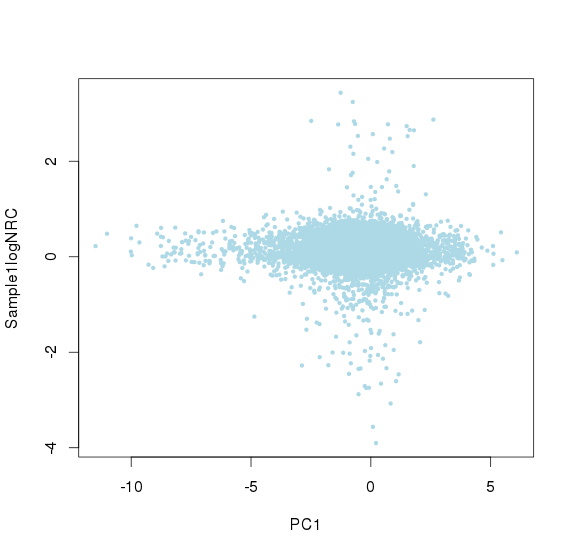
#qplot(S[tt,1],observations[tt,i],xlab="PC1",ylab="Sample1logNRC",alpha=0.1,colour=3)
#qplot(S[tt,2],observations[tt,i],xlab="PC2",ylab="Sample1logNRC",alpha=0.1,colour=3)
#qplot(S[tt,2],resi[tt],xlab="PC2",ylab="Sample1logNRC",alpha=0.1,colour=3)
resi<- observations[,i]-my.lm$coefficients[1]
for (PC in c(1:NUMBEROFPC)) {
resi<- resi-my.lm$coefficients[PC+1]*S[,PC]
}
#plotRatioFree(observations[,i],data$chr[indexNoNul],data$start[indexNoNul])
# #check sign:
## if (my.lm$coefficients[mainComp+1]<0) {resi<- -resi} - bug in version 5.5
observations[,i] <- resi
}
mu<-(baseLine[indexNoNul])
correctedObs[indexNoNul,]<-observations
data$IC1<-NA
if (NUMBEROFPC>1) {
data$IC2<-NA
}
if (NUMBEROFPC>2) {
data$IC3<-NA
}
tmp <- 1:NUMBEROFPC
data$IC1[indexNoNul] <- S[,mainComp]
tmp <- setdiff(tmp,mainComp)
if (NUMBEROFPC>1) {
data$IC2[indexNoNul]<- S[,tmp[1]]
}
if (NUMBEROFPC>2) {
data$IC3[indexNoNul]<- S[,tmp[2]]
}
} else {
baseLine <- correctedObs
data$IC1=correctedObs
}
#par(mfrow=c(1,2))
#plot(S[tt,1],resi[tt],xlab="PC1",ylab="Sample2logNRC",col="lightblue",pch=19,cex=0.5)
if (ncont >1){
#observations<-correctedObs[indexToFit,] #fit SD on indexToFit points:
#mu<- baseLine[indexToFit]
observations<-correctedObs[indexNoNul,] #fit SD on "indexNoNul" points starting from v.5.2
mu<- baseLine[indexNoNul]
#some control samples are noisier than others.., normalyze for it starting from version 4.0
sd.all <- mad(unlist(observations),na.rm=TRUE) #"mad" instead of "sd" starting from version 4.0 : 0.185[indexToFit] => 0.24[indexNoNul]
for (j in (1:(ncont))) { #starting from version 4.0 correct for variance
tt <- which(observations[,j]>=magicThreshold)
sd.j <- mad(unlist(observations[,j][tt]),na.rm=TRUE)
alph <- sd.j/sd.all
observations[,j]<-(observations[,j]-median(observations[,j],na.rm=TRUE))/alph+median(observations[,j],na.rm=TRUE) #use starting from version 4.0
}
# mu <- baseLine[indexToFit] #fit SD on "indexNoNul" points starting from v.5.2
#plot(S[,1],observations[,j],xlab="PC1",ylab="Sample1logNRC",col="lightblue",pch=19,cex=0.5)
totalPoints <- length(mu)
evalVal=50
if (totalPoints/evalVal<5) {
evalVal=10
}
numSeg=floor(totalPoints/evalVal)
possibleMu<-NULL
sigma<-NULL
observations <- observations[order(mu),]
mu <- mu[order(mu)]
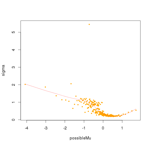
for (i in c(0:(numSeg-1))) {
possibleMu[i+1] <- mean(mu[(i*evalVal+1):(i*evalVal+evalVal)])
sigma[i+1]<-max(apply(observations[(i*evalVal+1):(i*evalVal+evalVal),],FUN=mad,MARGIN=2,center=0,na.rm=TRUE)) #"mad" instead of "sd" starting from version 4.0
}
#sigma.spl <- smooth.spline(possibleMu, sigma)
#data$sd<- predict(sigma.spl,baseLine)$y/max(apply(observations,FUN=mad,MARGIN=2,center=0,na.rm=TRUE))
sigma.spl <- loess(sigma~possibleMu, control = loess.control(surface = "direct"),degree=2) #loess starting from version 5.2
data$sd<- predict (sigma.spl,baseLine)/max(apply(observations,FUN=mad,MARGIN=2,center=0,na.rm=TRUE))
#plot(possibleMu,sigma,col="orange",cex=0.5,pch=19)
#lines(possibleMu,predict (sigma.spl,possibleMu),col="red",lwd=0.5)
tt <- which(data$sd<0)
if (length(tt)>0) {
cat(paste("Warning:",length(tt),"of amplicons have negative SD!!!"))
cat ("Will assign the maximum value of SD")
data$sd[tt] <- max(data$sd,na.rm=TRUE)
}
} else {
data$sd=rep(1,length(data$mean))
}
data$mean <- baseLine
data$mean[-indexNoNul]<-NA
#plot(baseLine[indexNoNul],data$sd[indexNoNul],col="orange",pch=19,cex=0.5)
#plot(baseLine[indexNoNul],data$sd[indexNoNul],col="orange",pch=19,cex=0.5,xlim=c(-2,3))
write.table(data,file=controlFile,quote=FALSE,sep=" ",row.names=FALSE)
参考资料
ONCOCNV文献:https://academic.oup.com/bioinformatics/article/30/24/3443/2422154
ONCOCNV代码:http://boevalab.com/ONCOCNV/