之前,浏览器一直出现缓冲问题,是配置文件设置的不对,解决方法如下:
1.到C:WindowsSystem32driversetc下找到host文件,并以文本方式打开,
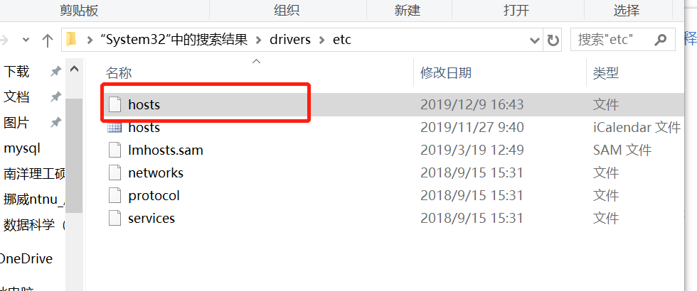
添加如下信息到hosts文件中:
52.84.246.90 d3c33hcgiwev3.cloudfront.net
52.84.246.252 d3c33hcgiwev3.cloudfront.net
52.84.246.144 d3c33hcgiwev3.cloudfront.net
52.84.246.72 d3c33hcgiwev3.cloudfront.net
52.84.246.106 d3c33hcgiwev3.cloudfront.net
52.84.246.135 d3c33hcgiwev3.cloudfront.net
52.84.246.114 d3c33hcgiwev3.cloudfront.net
52.84.246.90 d3c33hcgiwev3.cloudfront.net
52.84.246.227 d3c33hcgiwev3.cloudfront.net
2.刷新浏览器dns地址,ipconfig/flushdns
week01
1.1introduction
structure and usage of machine learning
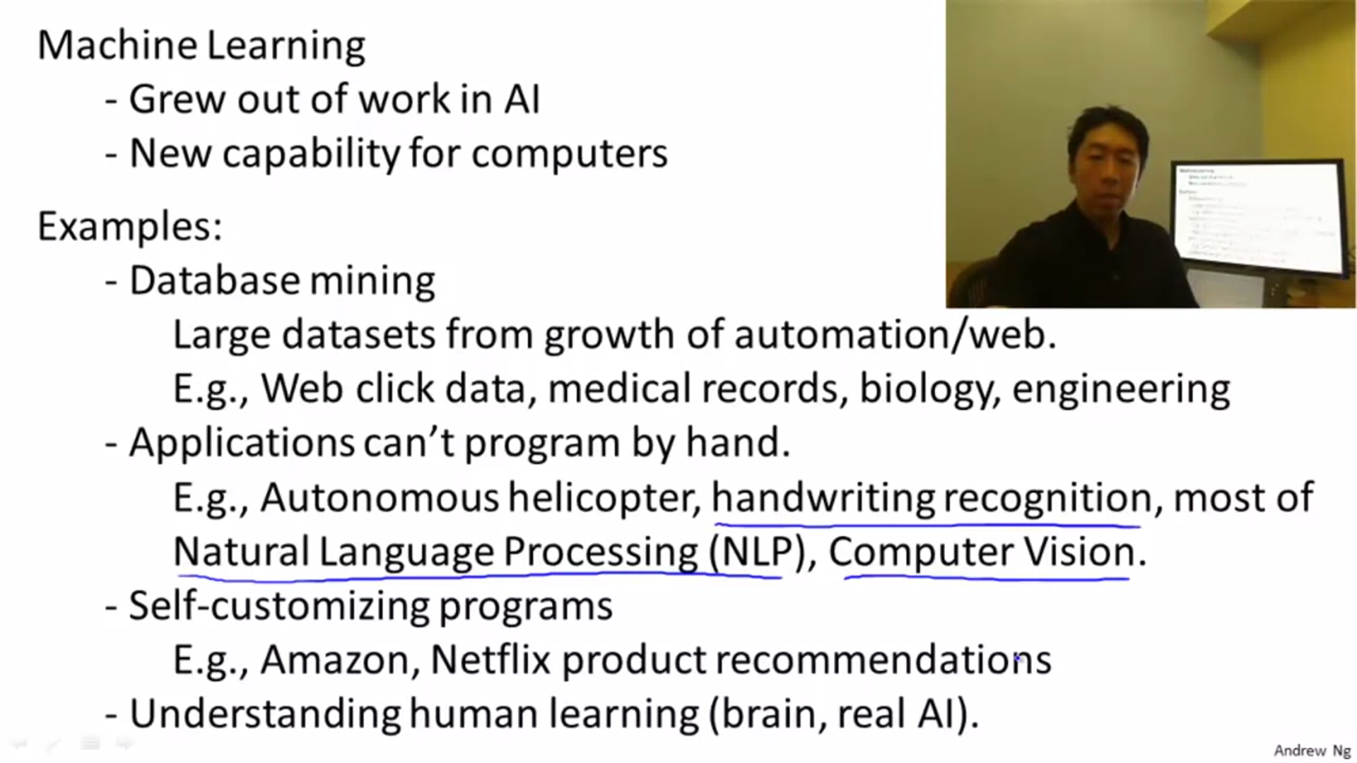
the definition of ML
A computer program is said to learn from experience E with respect to some class of tasks T and performance measure P, if its performance at tasks in T, as measured by P, improves with experience E
supervised learning
In supervised learning, we are given a data set and already know what our correct output should look like, having the idea that there is a relationship between the input and the output.
there are two types of supervised learning, that are regression and classification. one sign is whether the relationship of input and output is continuous.
unsupervised learning
there are no labels for the unsupervised learning, and we hope that the computer can help us to labels some databets.
1.2model and cost function
1.2.1模型导入:
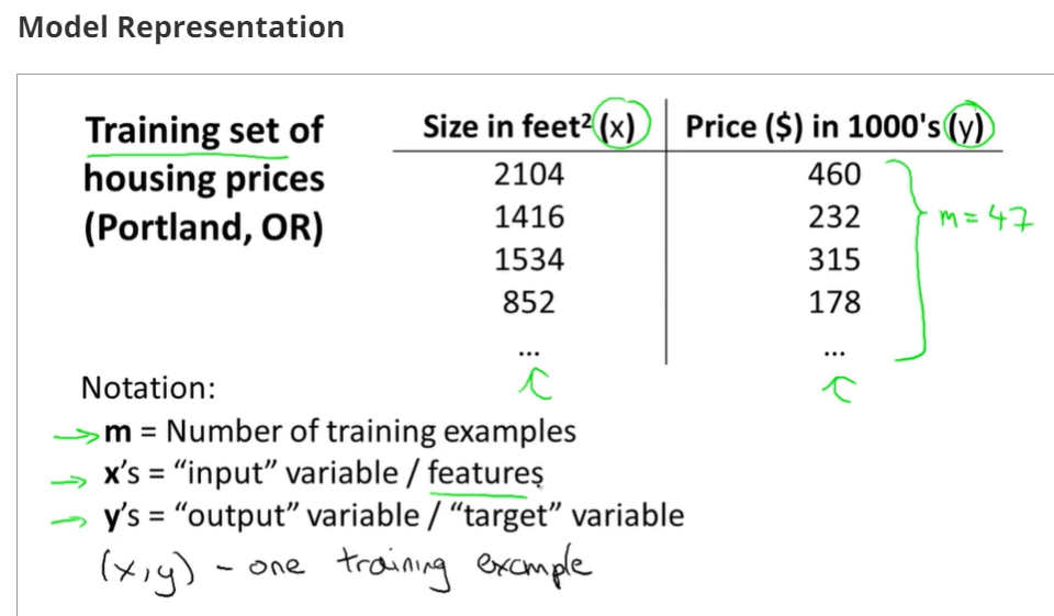
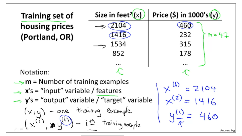
training examples(x(i),y(i)),i=1,2,3...,m,m is trainging set;
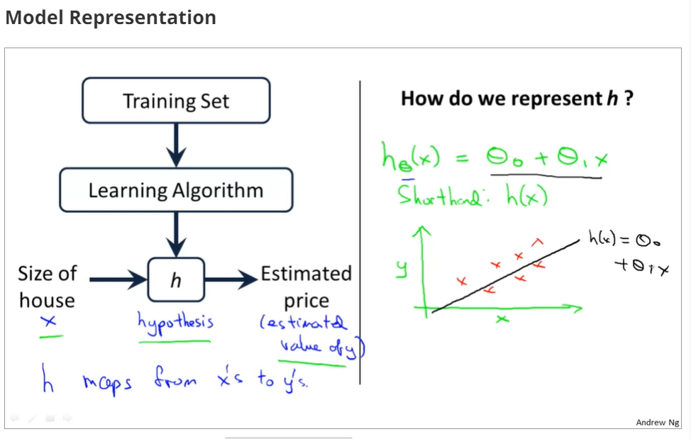
h(x) si a 'good' predictor for the goal of housing price of y,and h(x) here is called hypothesis;
if we are trying to predict the problem continuously, such as the housing price, we call the learning problem a regression problem.
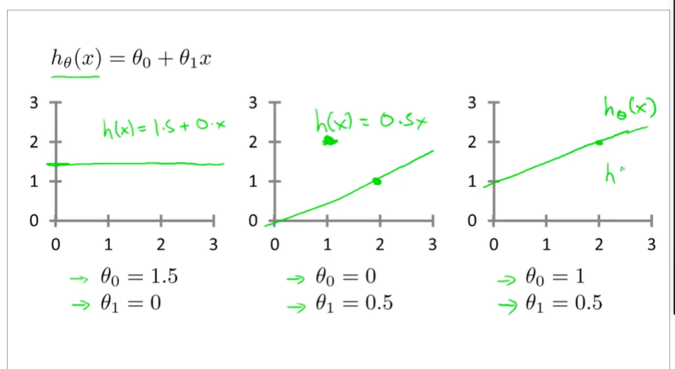
1.2.2some figures of linear regression
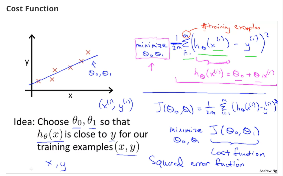
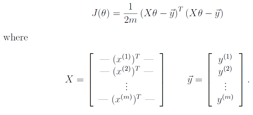
cost function
choose a suitable hθ(x) for making the error with y to the minimum
make a cost function
1.2.3cost function - intuition I
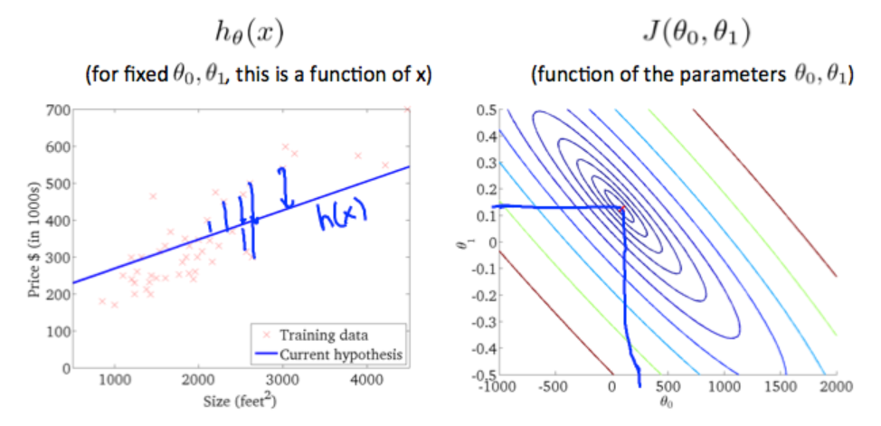
when θ0=0 and θ1=1,the cost function and function of the parameter is as below
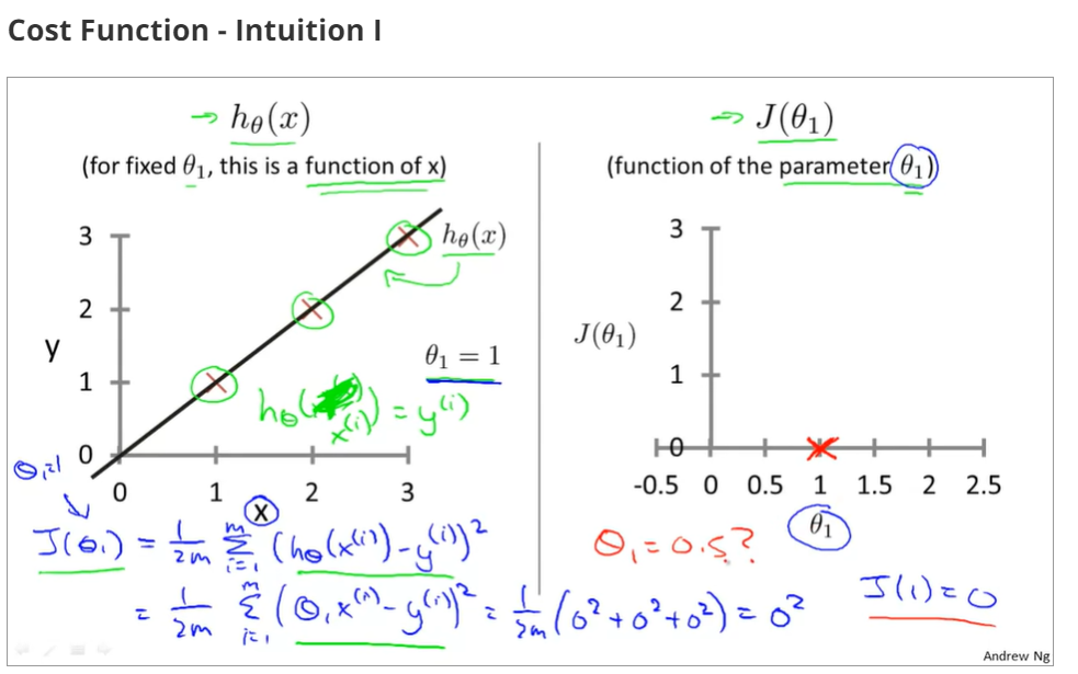
the relationship between the function of hypothesis function and the cost function, that is to say, there are different values of cost function that is corresponding to the the function of hypothesis
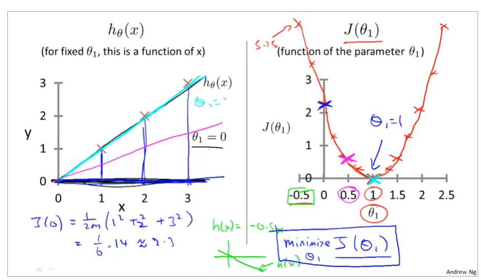
1.2.4Intuition II
now, it is fixed values of θ0,θ1,
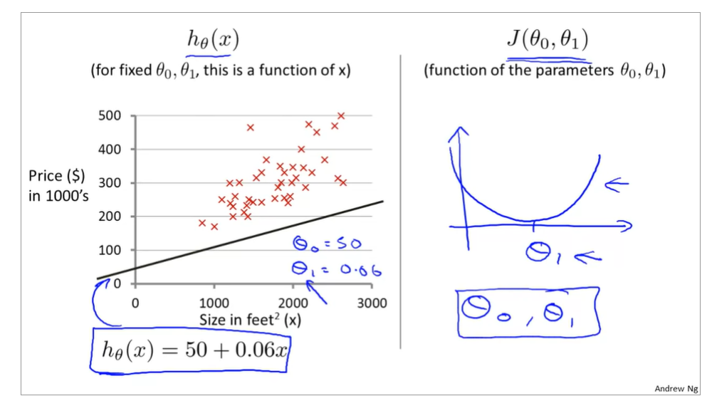
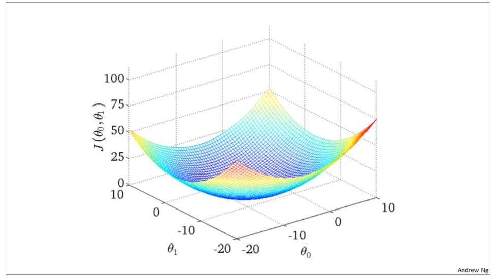
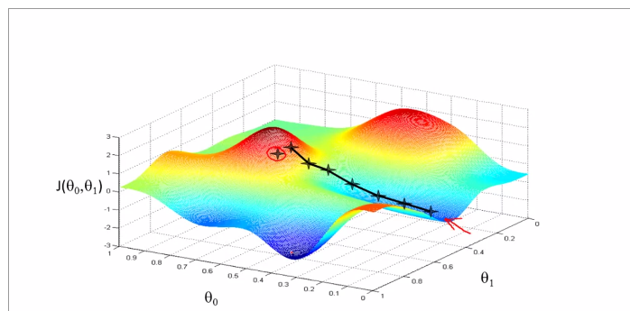
the curve face to the ground is the height of the J(θ0,θ1),we can see the description in the picture as below

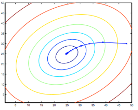
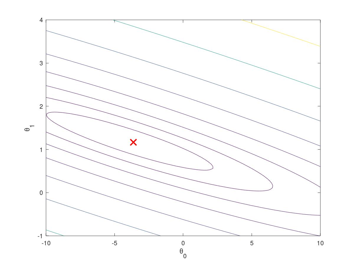
it is also called contour plots or contour figures to the left graph as below, and we can get the minimal result as much as possible,

1.2.5algorithm of function of hypothesis to minimize the cost function of J
the best algorithm is to find a function to make the value of cost function which is a second-order function to the minimum, and then the inner circle point is what we need get. It is also corresonding to the two values θ0 and θ1.

1.3parameter learning
1.3.1introduction of gradient descent
the theory of gradient descent, like a model going down the hill, it bases on the hypothesis function(theta0 and theta1), and the cost function J is bases on the hypothesis function graphed below.
the tangential line to a cost function is the black line which use athe derivative.
alpha is a parameter, which is called learning rate. A small alpha would result in a small step and a larger alpha would result in a larger step. the direction is taken by the partial derivative of J(θ0,θ1)
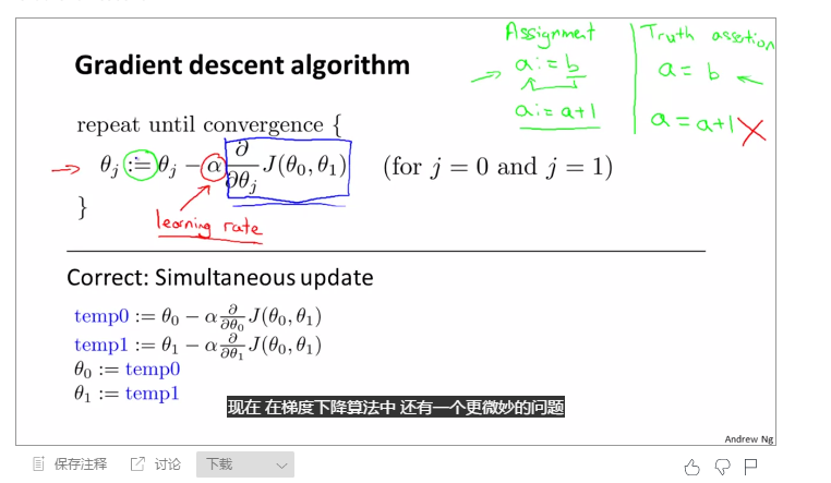
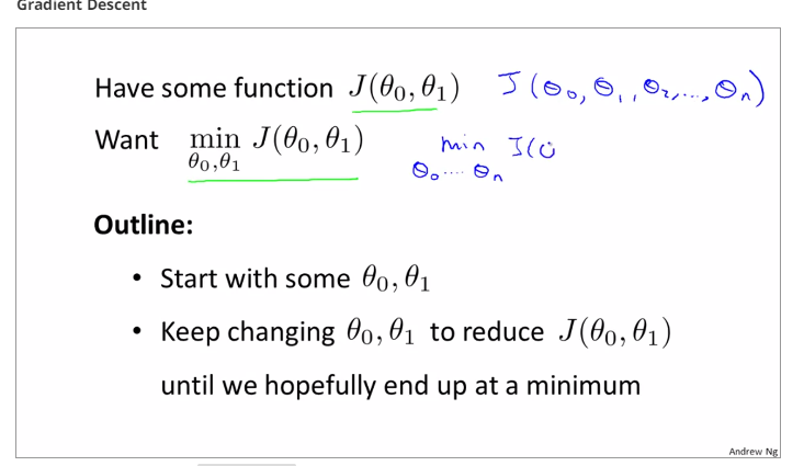
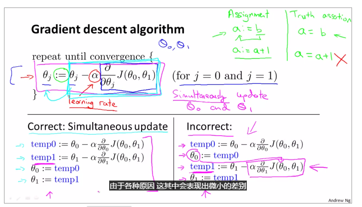
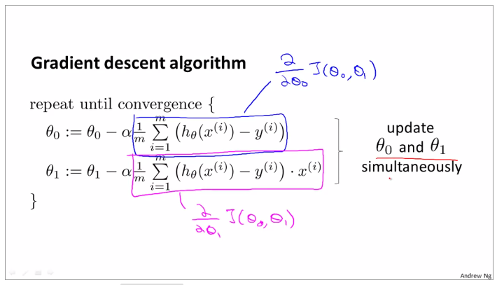
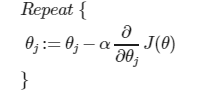
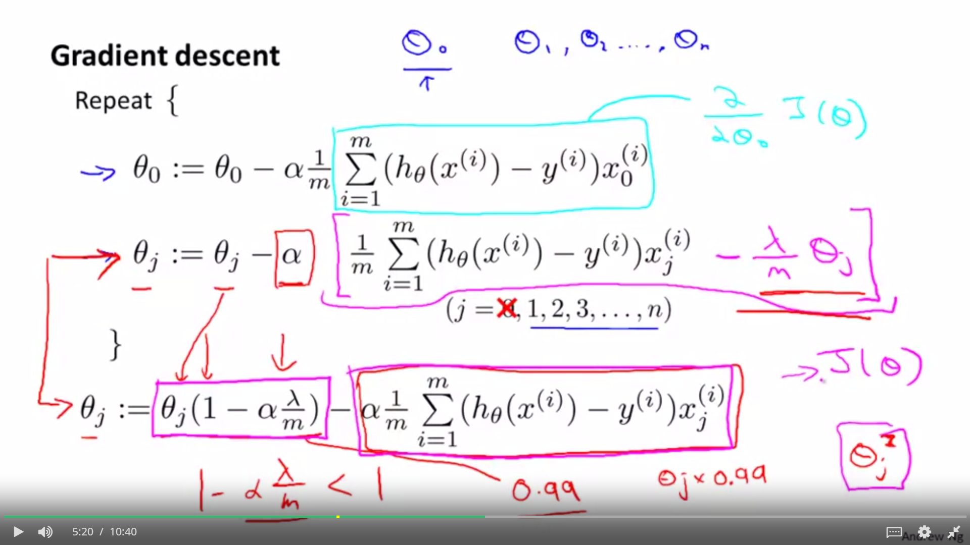
1.3.2OUTLINE OF THE GRADIENT DESCENT ALGORITHM
theta 0 and theta1 need update together, otherwise they will be replaced after operation, such as the line listed for theta 0, and next it is incorrect when replace the value of theta0 in the equation of temp1
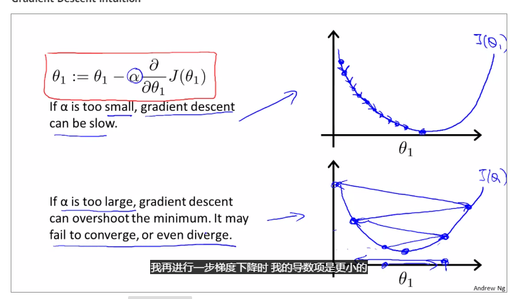
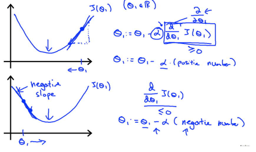
1.3.3Gradient Descent Intuition

if alpha is to small, gradient descent can be slow; and if alpha is to large, gradient descent can overshoot the minimum. may not be converge or even diverge.
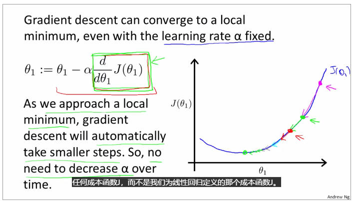
gradient descent can converge to a local minimum, whenever a learning rate alpha
gradient descent will automatically take smaller steps to make the result converge.
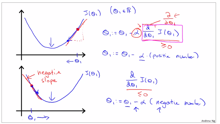
Use gradient descent to assure the change of theta, when the gradient is positive, the gradient descent gradually decrease and when the gradient is negative, the gradient descent gradually increase.
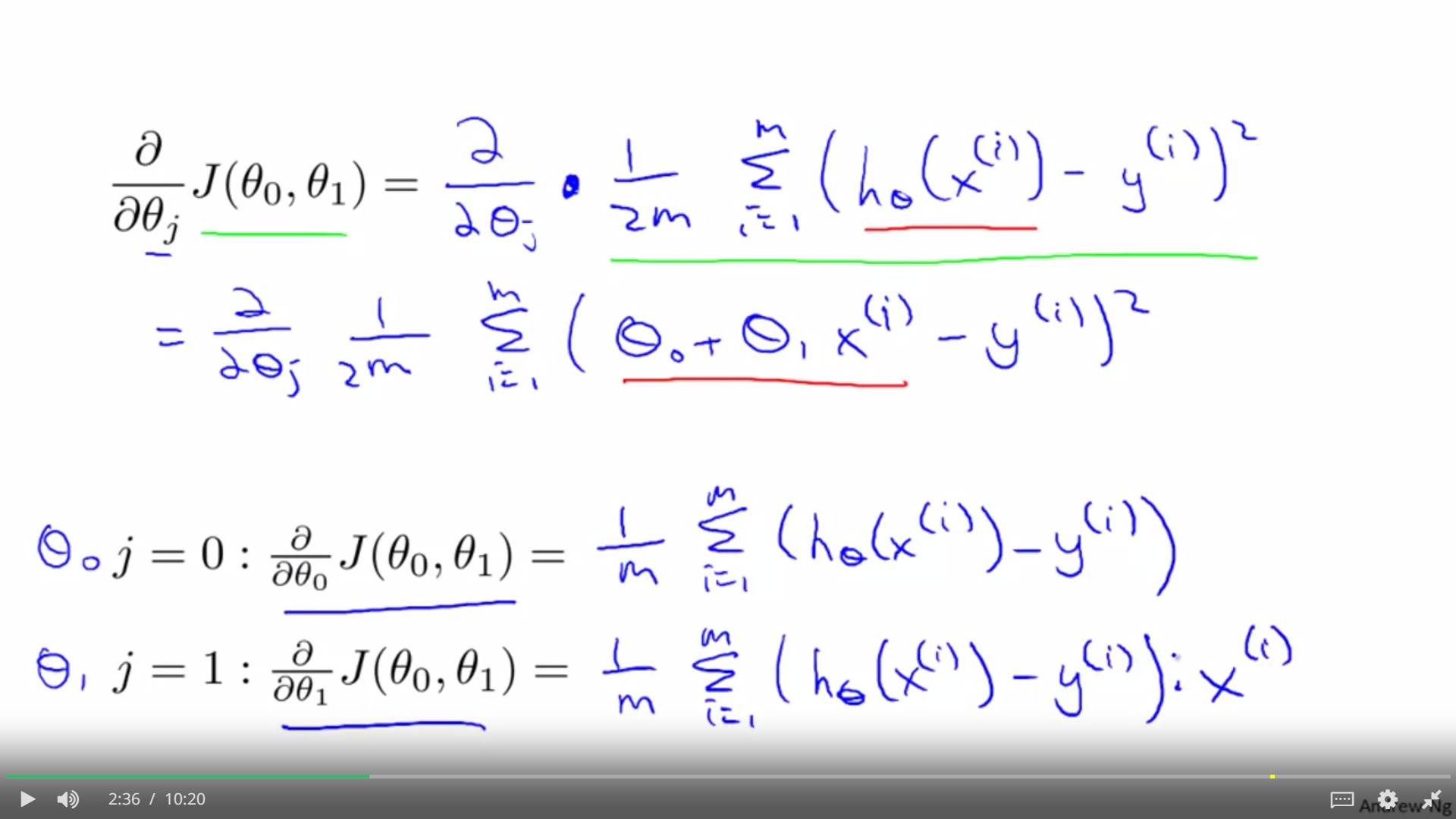
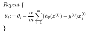
gradient for linear regression
partial derevative for theta0 and theta1
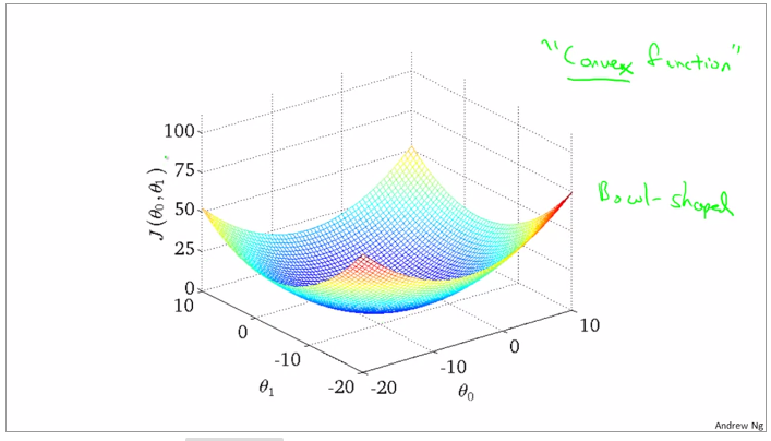
convex function and bowl shape


Batch gradient descent: every make full use of the training examples
gradient descent can be subceptible to local minima in general. gradient descent always converges to the global minimum.
review
vector is a matric which is nx1 matrix

R refers to the set of scalar real numbers.
Rn refers to the set of n-dimensional vectors of real numbers.
1.3.4Addition and scalar Multiplication
The knowledge here is similar with linear algebra, possibly there is no necessity to learn it.
1.3.5Matrix vector multiplication
The knowledge here is similar with linear algebra, possibly there is no necessity to learn it.
1.3.6Matrix Multiplication Properties
identity matrix
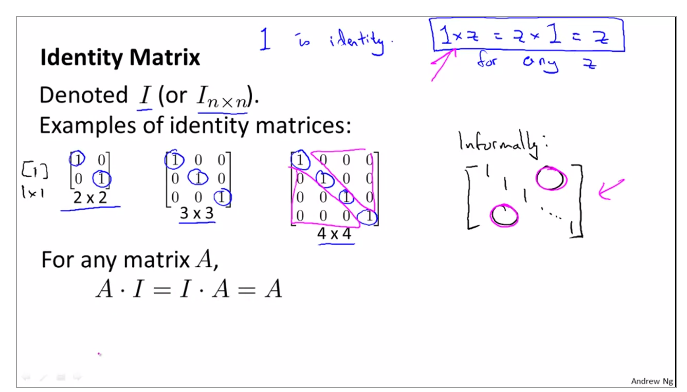
1.3.7review and review Inverse and Transpose of matrix
through computing, Matrix A multiply inverse A is not equal inverse A multiply Matrix A

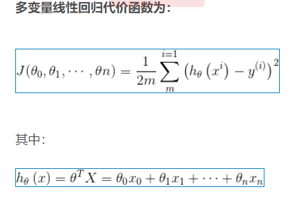
week02Linear regression
2.1Multiple features(variables)
2.1.1Multible linear regression
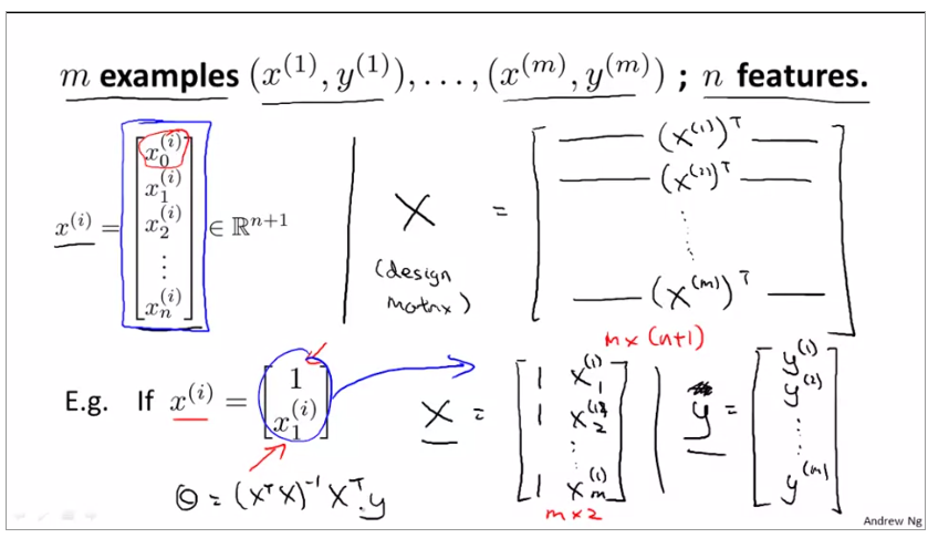
compute the value xj(i) = value of feature j in ith training sets
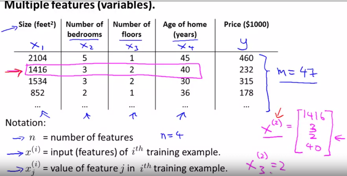
x3(2), x(2) means the line 2 and the x3 means the third number, that is to say it is 2.
put the hypothesis to the n order, that is multivariable form of the hypothesis function

to define the function hθ(x) of the n order, we need to make sense its meaning, there is an example to explain.

2.1.2gradient descent for multiple variables

2.1.3gradient descent in practice 1 - feature scaling
mean normalization

appropriate number of mean normalization can make the gradient descent more quick.
use xi := (xi - ui) / si,
where
is the average of all the values for feature (i) and si is the range of values (max - min), or si is the standard deviation.

is the average of all the values for feature (i) and si is the range of values (max - min), or si is the standard deviation.
2.1.4Graident descent in practice ii - learning rate
how to adjust the parameter of learning rate, it is also a type a debug, so may be use a 3 to multiply the original learning rate to adjust the value to the optimal.
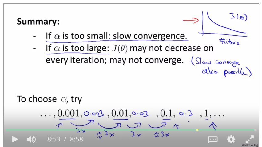
If J(θ) ever increases, then you probably need to decrease α.
when the curve is fluctuent, it needs a smaller learning rate.

To summarize:
If α is too small: slow convergence.
If α is too large: may not decrease on every iteration and thus may not converge.
2.1.5features and polynomial regression
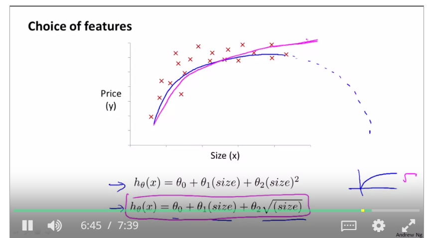
feature scaling is to find a new function that can fit the range of training examples, such as if the price is up to the feets ranging from 1 to 1000, and then the polinomial regression is used to change the type of the original function.
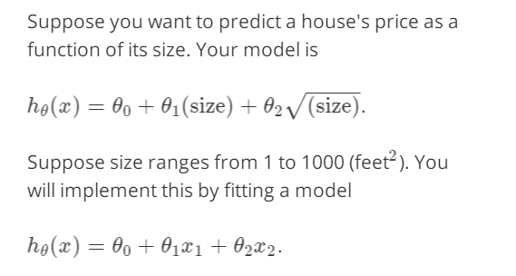
like this, we use two functions to compute the result, and x1 and x2 are that

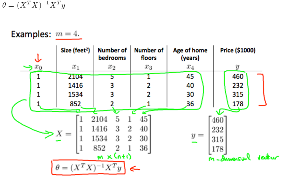
2.1.6Normal equation
for an example of normal equation
in programming:
x' means transpose x
pinv(x) means inverse Matrix
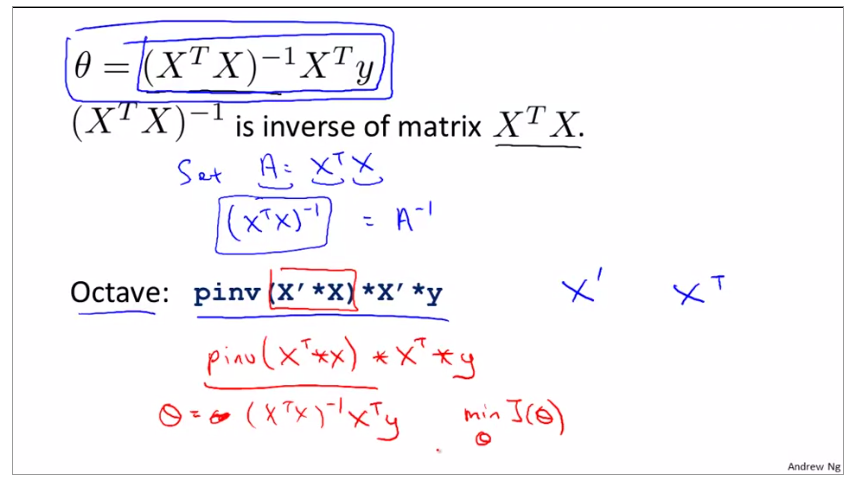
normal regression formula
the comparasion of the gradient descent and normal regression

2.1.7Normal Equation Noninvertibility
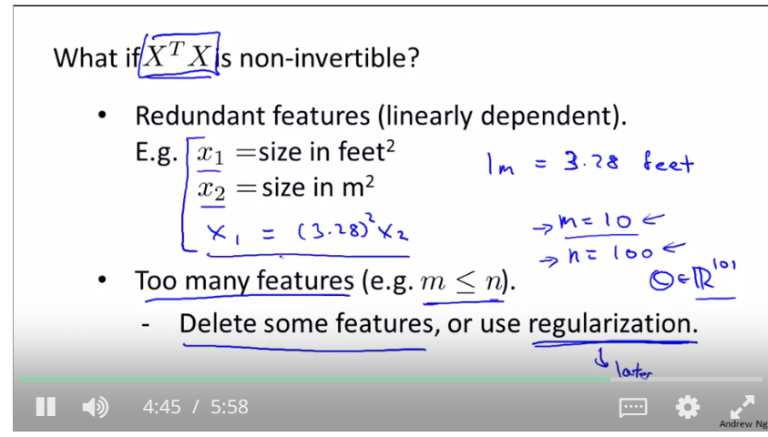
feature scaling: 特征缩放
normalized features:标准化特征
2.1.8practice of octive
some basic operation for octive, it is like some operations in matlab or python.numpy
2.1.9vectorization
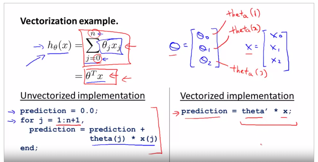
h(theta) is the original sythphasis function relate with theta0 and theta1, now use octave to vectorize it. prediction = theta' * x + theta(j) * x(j)
its programming in C++ below
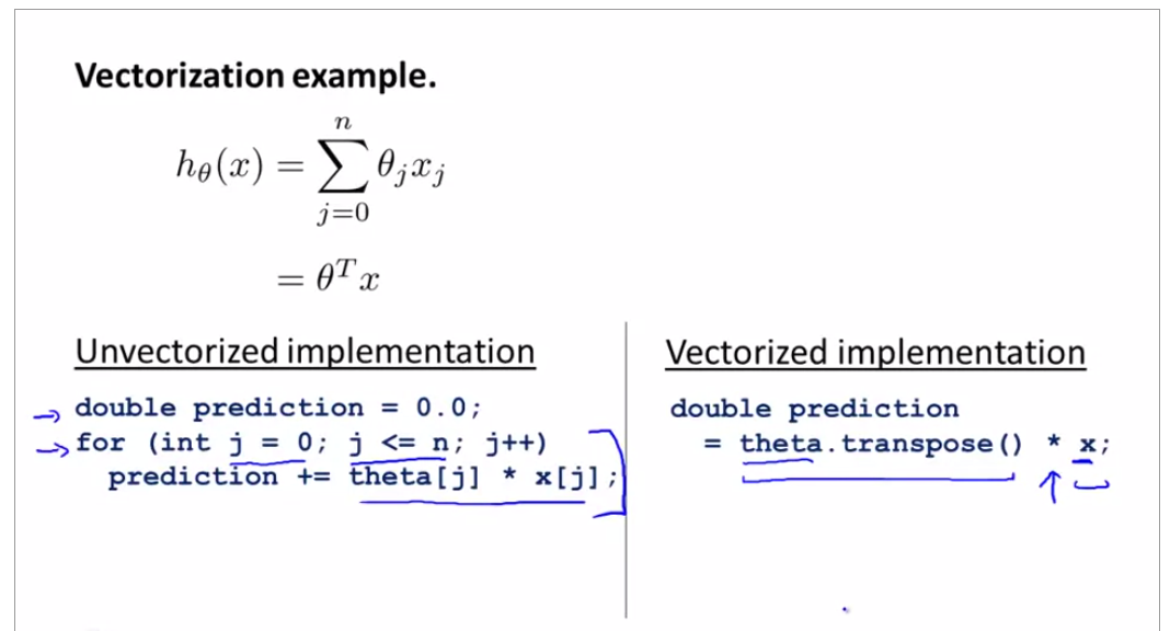
download octave to programming, GNU octave docs is here.
2.2homeworkweek02
part1 linear regression with one variable
2.2.1input the data
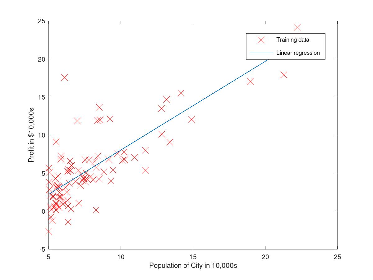
create a scatter plot to represent the plotData on the column1 and column2


clear ; close all; clc

%% ==================== Part 1: Basic Function ====================
% Complete warmUpExercise.m
fprintf('Running warmUpExercise ...
');
fprintf('5x5 Identity Matrix:
');
warmUpExercise()

fprintf('Program paused. Press enter to continue.
');
pause;

%% ======================= Part 2: Plotting =======================
fprintf('Plotting Data ...
')
data = load('ex1data1.txt');
X = data(:, 1); y = data(:, 2);
m = length(y); % number of training examples

% Plot Data
% Note: You have to complete the code in plotData.m
plotData(X, y);

2.2.2 calculate the gradientDescent and computeCost
when fix the function of gradientDescent and computeCost, we can see the files as below,
gradientDescent:
function [theta, J_history] = gradientDescent(X, y, theta, alpha, num_iters)
%GRADIENTDESCENT Performs gradient descent to learn theta
%   theta = GRADIENTDESCENT(X, y, theta, alpha, num_iters) updates theta by
%   taking num_iters gradient steps with learning rate alpha

% Initialize some useful values
m = length(y); % number of training examples
J_history = zeros(num_iters, 1);

for iter = 1:num_iters

    % ====================== YOUR CODE HERE ======================
    % Instructions: Perform a single gradient step on the parameter vector
    %               theta.
    %
    % Hint: While debugging, it can be useful to print out the values
    %       of the cost function (computeCost) and gradient here.
    %

    theta = theta - X'*(X*theta-y)*alpha/m;


    % ============================================================

    % Save the cost J in every iteration
    J_history(iter) = computeCost(X, y, theta);

end

end


computeCost:
function J = computeCost(X, y, theta)
%COMPUTECOST Compute cost for linear regression
%   J = COMPUTECOST(X, y, theta) computes the cost of using theta as the
%   parameter for linear regression to fit the data points in X and y

% Initialize some useful values
m = length(y); % number of training examples

% You need to return the following variables correctly
J = 0;

% ====================== YOUR CODE HERE ======================
% Instructions: Compute the cost of a particular choice of theta
%               You should set J to the cost.

h = X*theta;
squerror = (h-y).^2;
J = sum(squerror)*1/(2*m);


% =========================================================================

end
so the testing result is showed when ex1 file is compiled.
Testing the cost function ...
With theta = [0 ; 0]
Cost computed = 32.072734
Expected cost value (approx) 32.07
2.2.3upload the results
when it comes to upload the files to the platform of coursera, we need put the foldbox into the ex1, and then write the submit on the command line, then use the E-mail when you registered on the coursera and the Identification code to identify your information. finally there are lines on the command line and you can receive your scores.
== Submitting solutions | Linear Regression with Multiple Variables...
Login (email address): 386460856@qq.com
Token: NIJj0TBYuxghfz3n
warning: findstr is obsolete; use strfind instead
warning: strmatch is obsolete; use strncmp or strcmp instead
==
==                                   Part Name |     Score | Feedback
==                                   --------- |     ----- | --------
==                            Warm-up Exercise |  10 /  10 | Nice work!
==           Computing Cost (for One Variable) |  40 /  40 | Nice work!
==         Gradient Descent (for One Variable) |  50 /  50 | Nice work!
==                       Feature Normalization |   0 /   0 |
==     Computing Cost (for Multiple Variables) |   0 /   0 |
==   Gradient Descent (for Multiple Variables) |   0 /   0 |
==                            Normal Equations |   0 /   0 |
==                                   --------------------------------
==                                             | 100 / 100 |
==
2.2.4calculate the parameter of theta1 and theta2 as well as debugging
After fixing the function of gradientDescent
theta = gradientDescent(X, y, theta, alpha, iterations);
we could get the data of theta
theta

and the result is below,
theta =

  -3.6303
   1.1664
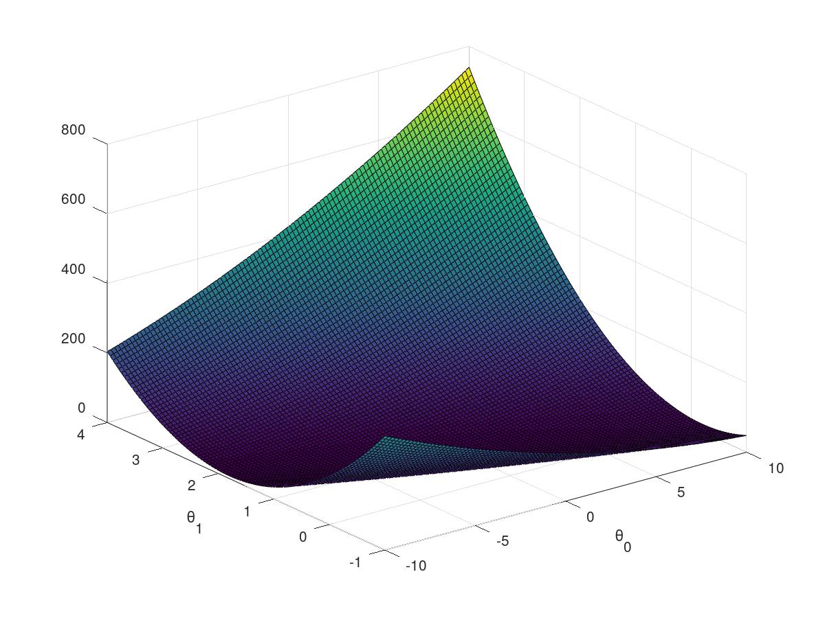
2.2.5visualing the J(theta)
3D array of J(theta) value and its 2D
theta0_vals = linspace(-10, 10, 100);
theta1_vals = linspace(-1, 4, 100);

J_vals = zeros(length(theta0_vals), length(theta1_vals));

for i = 1:length(theta0_vals)
    for j = 1:length(theta1_vals)
      t = [theta0_vals(i); theta1_vals(j)];
      J_vals(i,j) = computeCost(X, y, t);
    end
end


J_vals = J_vals';
figure;
surf(theta0_vals, theta1_vals, J_vals)
xlabel('	heta_0'); ylabel('	heta_1');

figure;
contour(theta0_vals, theta1_vals, J_vals, logspace(-2, 3, 20))
xlabel('	heta_0'); ylabel('	heta_1');
hold on;
plot(theta(1), theta(2), 'rx', 'MarkerSize', 10, 'LineWidth', 2);
part2 linear regression with multible variable(regularization)
2.3.1feature Normalization
fix the code in the corresponding section
mu = mean(X);
sigma = std(X);
X_norm = (X - mu) ./ sigma
so that we get the value after feature normalization.
since our function of gradientDescent has considered the situation of multivariable, so we do not calculate it again. Just copy it from the previous file
theta = theta - X'*(X*theta-y)*alpha/m;
and everytime the cost function can be written by the form of vectorization as followed.
2.3.2different learning rate alpha
when it comes to the situation of the multivariable, introducing the normal equation is beneficial to adjust the parameters of theta.
the normal equation is to find a cost function to minimize the parameters of theta.
e10=10^10
then we set three different numbers of alpha,respectively alpha 0.03,0.1,0.3 to get three figures
% Choose some alpha value
alpha = 0.01;
num_iters = 400;

% Init Theta and Run Gradient Descent
theta = zeros(3, 1);
[theta, J1] = gradientDescentMulti(X, y, theta, alpha, num_iters);

% Choose some alpha value
alpha = 0.03;

% Init Theta and Run Gradient Descent
theta = zeros(3, 1);
[theta, J2] = gradientDescentMulti(X, y, theta, alpha, num_iters);

% Choose some alpha value
alpha = 0.1;

% Init Theta and Run Gradient Descent
theta = zeros(3, 1);
[theta, J3] = gradientDescentMulti(X, y, theta, alpha, num_iters);

% Plot the convergence graph
figure;
plot(1:numel(J1),J1, 'b', 'LineWidth', 2);
hold on;
plot(1:numel(J2),J2, 'r', 'LineWidth', 2);
plot(1:numel(J3),J3, 'k', 'LineWidth', 2);

2.3.3normal equation
closed-form solution to linear regression is
![]()
cost function with linear regression with multi-variable
用gradient Descent要特征数据缩放,而使用normal equation则不用缩放
为什么?
特征缩放可以理解为平时我们常说的归一化,使得变量x的范围落在区间[-1,1]里,一方面对多个范围差别很大的特征量可以更直观的表示,另一方面当使用梯度下降算法时可以更快的收敛,即迭代次数少
特征缩放的使用是有范围的,当-3<x<3 or -1/3<x<1/3属于可接受的范围,如果-100<x<100 or -0.0001<x<0.0001,特征缩放带来的误差较大,不可使用
所以总结,在梯度下降法算线性回归问题时,主要可以保证代价函数收敛,如果不缩放,X过大,导致cost function 发散。
梯度下降法的预测价格方程是
price = [1 (1650-mu(1))/sigma(1) (3-mu(1))/sigma(1)]*theta %price = 假设函数h = X'*theta
标准差=方差的算术平方根=s=sqrt(((x1-x)^2 +(x2-x)^2 +......(xn-x)^2)/(n-1))
有归一化后,基本上可以控制X在-3<x<3 or -1/3<x<1/3。
正规化的预测价格方程是
price = [1 1650 3] * theta
预测到的价格也接近的
Running gradient descent ...
Theta computed from gradient descent:
 340412.659574
 110631.048958
 -6649.472950

price =  308309.23682
Predicted price of a 1650 sq-ft, 3 br house (using gradient descent):
 $308309.236819
Program paused. Press enter to continue.
Solving with normal equations...
Theta computed from the normal equations:
 89597.909543
 139.210674
 -8738.019112

price =  293081.46433
Predicted price of a 1650 sq-ft, 3 br house (using normal equations):
 $293081.464335
week03 Classification and representation
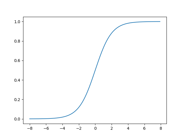
3.1sigmoid function
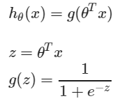
sigmoid python代码:
import matplotlib.pyplot as plt
import numpy as np

def sigmoid(x):
    return 1. /(1. +  np.exp(-x))

def figure_sigmoid():
    x = np.arange(-8,8,0.1)
    y = sigmoid(x)
    plt.plot(x,y)
    plt.show()

if __name__ == "__main__":
    figure_sigmoid()
3.1.1To predict linear decision boundary
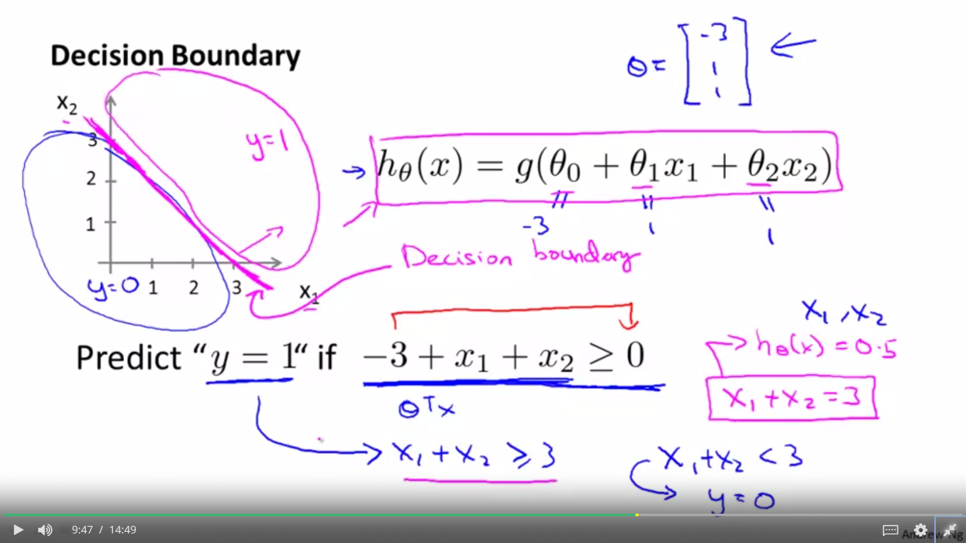
if we need to predict when the y is equal to 1, just make the g(x) ≥0, that is to say to make the g(theta 0 + theta 1*x1 + theta 2*x2≥0). So we could figure out the probability of (y=1). Meanwhile, it is the same method to calculate the probability of (y=0)
3.1.2To predict non-linear decision boundary
such as circle of radius 1, when the g(x) is more than 1, then the probability of y is equal to 1

3.2the definition of cost function

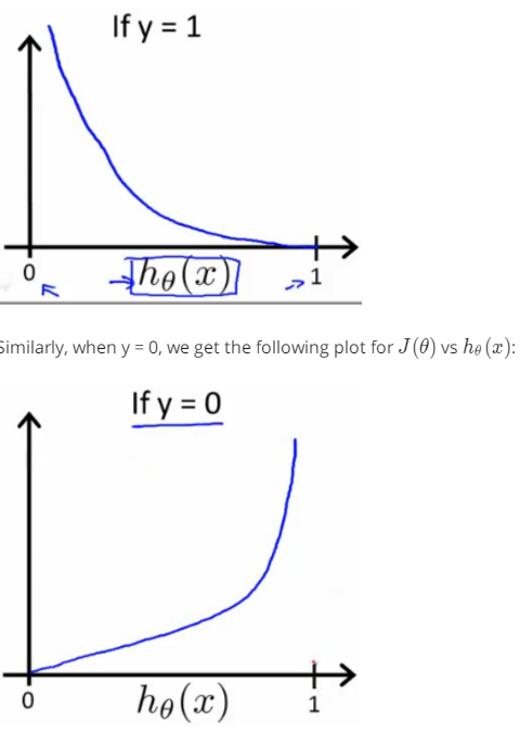
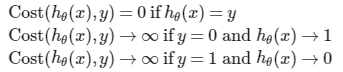
write the cost function in this way is to guarantee the figure of function with convex.
3.2.1simplified cost function and gradient descent
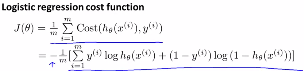
the deduction of logistic regression cost function

and extend to the n order
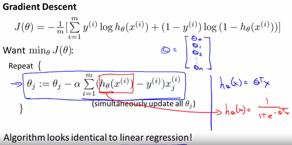
implement gradient descent to the logistic regression, same as the gradient with linear regression, but different.
the difference between Linear Regression and Logistic Regression
point1: function is different, LR is used for Classification, but linear regression is for Regression;
point2: equation is different, LR is a polynomial function, but linear regression is a sigmoid function;
point3: cost function is different, LR is a function described in this chapter of topic2 week03,and it is same as below![]()
but linear regression is a bowl function when there are two parameters or more, showed in the chapter02 topic03, week02, its feature like f(theta)=theta0+ theta1*x+theta2*x+...
the gradient descent is always like this one, if the J(theta) is determined.
this function is identical to the one in the linear regression, all values in theta should be updated after one round.
a vectorized implementation is
![]()
3.3advance optimization algorithm and its method
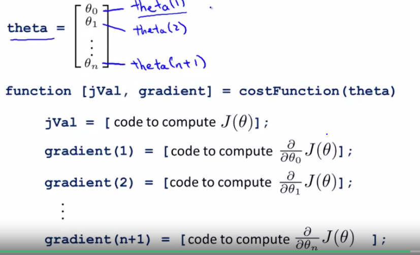
how to use programming language to compute equation of cost function and gradient
when it comes to logistic regression, the cost function and gradient are as below. Note that the number must start from 1, when variable parameters of theta are defined.
three other convergent algorithm, such as "Conjugate gradient",BFGS,L-BFGS
3.4how to choose classifiers
if there are 3 classes, we can pick up 3 classifiers. just like the picture, it shows the deduction of classification.

3.5using regularizaition to solve the problem of overfitting
3.6homeworkweek03
part1logistic regression
3.6.1input the data saved at plotData
plotData.m文件内容:
figure; hold on;

positive = find(y==1);
negative = find(y==0);
plot(X(positive,1),X(positive,2),"r+");
plot(X(negative,1),X(negative,2),"bo");

hold off;


ex2.m文件内容
hold on;
% Labels and Legend
xlabel('Exam 1 score')
ylabel('Exam 2 score')

% Specified in plot order
legend('Admitted', 'Not admitted')
hold off;

fprintf('
Program paused. Press enter to continue.
');
pause;

3.6.2iwrite the sigmoid function
g = zeros(size(z));
a = -z;
b = e.^a;
c = 1 + b;
g = 1 ./ c;
3.6.3write the cost function
乘除运算时,对于向量而言要加".",加减运算时不要
function [J, grad] = costFunction(theta, X, y)

m = length(y); % number of training examples
J = 0;
grad = zeros(size(theta));
J = -1/m * ( y'*log(sigmoid(X*theta)) + (1-y)'*log(1-sigmoid(X*theta)) );
grad = 1/m * X' * (sigmoid(X*theta)-y)

end
result of the cost:
Expected cost (approx): 0.693
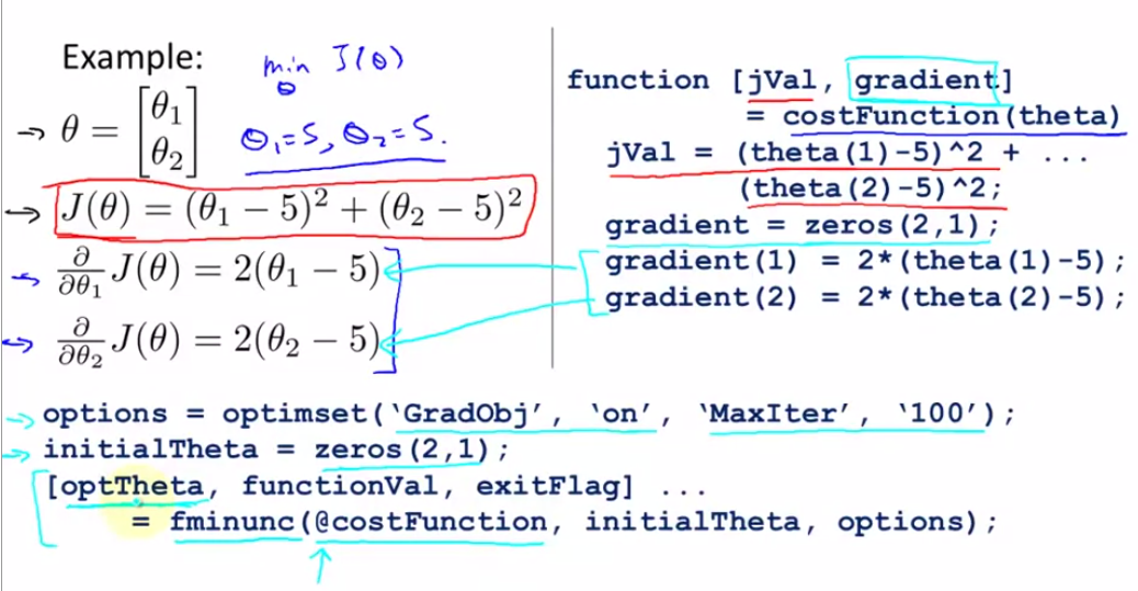
3.6.3get the learning parameters using fminunc as well as theta
fminunc函数作用:
using fminunc, we do not have to write any loops ourself or
set a learning rate like you did for gradient descent
we can get the cost value using fminunc function
Cost at theta found by fminunc: 0.203498
Expected cost (approx): 0.203
we can get the theta using fminunc function
theta =
  -25.16127
    0.20623
    0.20147
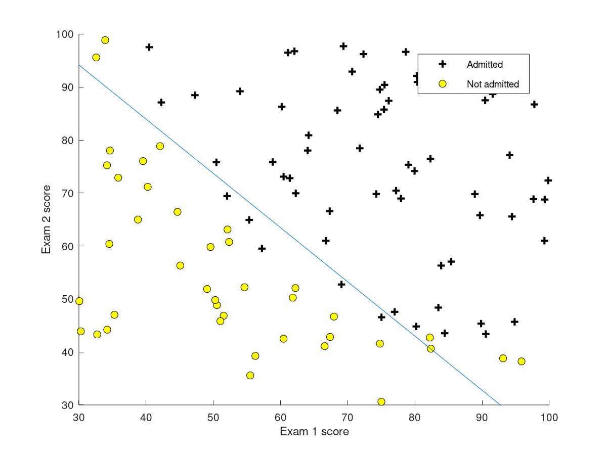
3.6.4using the theta above to plot the figure of DecisionBoundary
function plotDecisionBoundary(theta, X, y)
%PLOTDECISIONBOUNDARY Plots the data points X and y into a new figure with
%the decision boundary defined by theta
%   PLOTDECISIONBOUNDARY(theta, X,y) plots the data points with + for the
%   positive examples and o for the negative examples. X is assumed to be
%   a either
%   1) Mx3 matrix, where the first column is an all-ones column for the
%      intercept.
%   2) MxN, N>3 matrix, where the first column is all-ones

% Plot Data
plotData(X(:,2:3), y);
hold on

if size(X, 2) <= 3
    % Only need 2 points to define a line, so choose two endpoints
    plot_x = [min(X(:,2))-2,  max(X(:,2))+2];

    % Calculate the decision boundary line
    plot_y = (-1./theta(3)).*(theta(2).*plot_x + theta(1));

    % Plot, and adjust axes for better viewing
    plot(plot_x, plot_y)

    % Legend, specific for the exercise
    legend('Admitted', 'Not admitted', 'Decision Boundary')
    axis([30, 100, 30, 100])
else
    % Here is the grid range
    u = linspace(-1, 1.5, 50);
    v = linspace(-1, 1.5, 50);

    z = zeros(length(u), length(v));
    % Evaluate z = theta*x over the grid
    for i = 1:length(u)
        for j = 1:length(v)
            z(i,j) = mapFeature(u(i), v(j))*theta;
        end
    end
    z = z'; % important to transpose z before calling contour

    % Plot z = 0
    % Notice you need to specify the range [0, 0]
    contour(u, v, z, [0, 0], 'LineWidth', 2)
end
hold off

end
and the figure that is training data with decision boundary are showed as below.
3.6.5evaluating logistic regression
应用训练好的模型参数
这里要取整,所以用到round()函数
p = round(sigmoid(X*theta));
get the result as below,
For a student with scores 45 and 85, we predict an admission probability of 0.776289
Expected value: 0.775 +/- 0.002

Train Accuracy: 89.000000
Expected accuracy (approx): 89.0
线性回归+正规化线性回归 for regression
逻辑回归+正规化逻辑回归 for classification
part2logistic regression with normal regularization
3.6.6regularized logistic regression
at first, input the data from the file to ex2data2.txt, sot that we can get the plot of training set. It is not a linear decision boundary but a circle decision boundary.
data = load('ex2data2.txt');
X = data(:, [1, 2]); y = data(:, 3);

plotData(X, y);

hold on;

xlabel('Microchip Test 1')
ylabel('Microchip Test 2')

legend('y = 1', 'y = 0')
hold off;

3.6.7cost function and gradient
这里最需要注意的是区分theta(1)和theta(2:n+1)这一种情况,当Θ0时,即theta(1)情况下,算grad(1,:),X=X(:,1);当Θ1-n时,即theta(2)-theta(n+1)情况下,算grad(2:end,:),X=X(:,2:end)。
代码如下:
function [J, grad] = costFunctionReg(theta, X, y, lambda)

m = length(y); % number of training examples

J = 0;
grad = zeros(size(theta));

J = -(1/m) * ((y')*log(sigmoid(X*theta))+(1-y)'*log(1-sigmoid(X*theta))) + (lambda/(2*m))*sum(theta(2:end).^2);
grad(1,:) = 1/m * (X(:,1)'*(sigmoid(X*theta)-y));
grad(2:end,:) = 1/m * (X(:,2:end)'*(sigmoid(X*theta)-y)) + (lambda/m)*theta(2:end);

end
可以得到真实的cost and gradient和expected cost and gradient(using fminunc)
Cost at initial theta (zeros): 0.693147
Expected cost (approx): 0.693

Gradient at initial theta (zeros) - first five values only:
 0.008475
 0.018788
 0.000078
 0.050345
 0.011501
Expected gradients (approx) - first five values only:
 0.0085
 0.0188
 0.0001
 0.0503
 0.0115

Cost at test theta (with lambda = 10): 3.164509
Expected cost (approx): 3.16
Gradient at test theta - first five values only:
 0.346045
 0.161352
 0.194796
 0.226863
 0.092186
Expected gradients (approx) - first five values only:
 0.3460
 0.1614
 0.1948
 0.2269
 0.0922
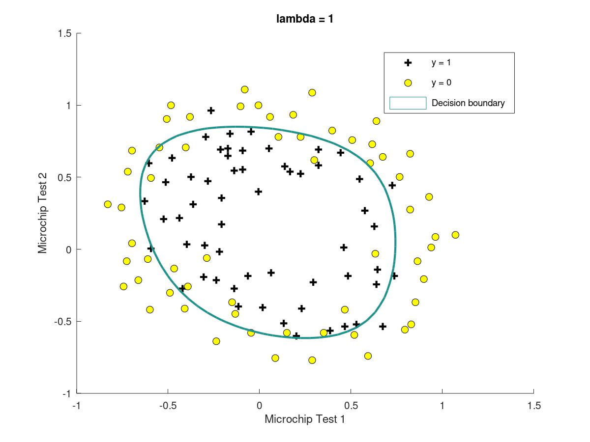
3.6.7plot the decision boundary
plotDecisionBoundary.m这个文件里if中包含了linear的情况,而else里包含的是non-linear的情况,figure如下

3.6.7three different situation with different lambda
when there is a larger lambda, it is likely to get a figure with underfitting result; for lambda=100
when there is a suitable lambda, it is likely to get a figure with good result; for lambda=1
when there is a smaller lambda, it is likely to get a figure with overfitting result; for lambda=0