1. Shrinkage(缩减) Methods
当特征比样本点还多时(n>m),输入的数据矩阵X不是满秩矩阵,在求解(XTX)-1时会出现错误。接下来主要介绍岭回归(ridge regression)和前向逐步回归(Foward Stagewise Regression)两种方法。
1.1 岭回归(ridge regression)
简单来说,岭回归就是在矩阵XTX上加上一个![]() 从而使得矩阵非奇异,进而能进行求逆。其中矩阵I是一个单位矩阵,
从而使得矩阵非奇异,进而能进行求逆。其中矩阵I是一个单位矩阵,![]() 是一个调节参数。
是一个调节参数。
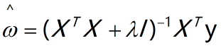
岭回归的回归系数计算公式为:
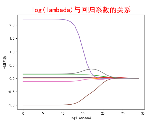
岭回归最先用来处理特征数多于样本的情况,现在也用于在估计中加入偏差,来得到更好的估计。当![]() =0时,岭回归和普通线性回归一样,当
=0时,岭回归和普通线性回归一样,当![]() 趋近于正无穷时,回归系数接近于0。可以通过交叉验证的方式得到使测试结果最好的
趋近于正无穷时,回归系数接近于0。可以通过交叉验证的方式得到使测试结果最好的![]() 值。
值。
岭回归代码:
 1 # encoding: utf-8
 2 '''
 3 @Author: shuhan Wei
 4 @File: ridgeRegression.py
 5 @Time: 2018/8/24 11:16
 6 '''
 7 import numpy as np
 8 import matplotlib.pyplot as plt
 9
10 def loadDataSet(fileName):
11     numFeat = len(open(fileName).readline().split('\t')) - 1
12     dataMat = []; labelMat = []
13     fr = open(fileName)
14     for line in fr.readlines():
15         lineArr = []
16         curLine = line.strip().split('\t')
17         for i in range(numFeat):
18             lineArr.append(float(curLine[i]))
19         dataMat.append(lineArr)
20         labelMat.append(float(curLine[-1]))
21     return dataMat, labelMat
22
23
24 """
25     函数说明:岭回归函数 w=(XT*X+lamI)-1 * XT*y
26     Parameters:
27         xMat - x数据集
28         yMat - y数据集
29         lam - 用户自定义参数
30     Returns:
31         ws  - 回归系数
32 """
33 def ridgeRegres(xMat, yMat, lam=0.2):
34     xTx = xMat.T * xMat
35     denom = xTx + np.eye(np.shape(xMat)[1]) * lam
36     if np.linalg.det(denom) == 0.0:
37         print("The matrix is singular, cannot do inverse")
38         return
39     ws = denom.I * (xMat.T * yMat)
40     return ws
41
42
43 """
44     函数说明:测试岭回归
45     Parameter:
46         xArr - x数据集矩阵
47         yArr - y数据集矩阵
48     Returns:
49         wMat - 回归系数矩阵,30组系数
50 """
51 def ridgeTest(xArr, yArr):
52     xMat = np.mat(xArr); yMat = np.mat(yArr).T
53     #对数据进行标准化处理
54     yMean = np.mean(yMat, 0)
55     yVar = np.var(yMat,0)
56     yMat = yMat - yMean
57     xMeans = np.mean(xMat,0)    #行操作
58     xVar = np.var(xMat, 0)
59     xMat = (xMat - xMeans) / xVar
60     numTestPts = 30 # 在30个不同lambda值下
61     wMat = np.zeros((numTestPts, np.shape(xMat)[1]))  #系数矩阵
62     for i in range(numTestPts):
63         ws = ridgeRegres(xMat, yMat, np.exp(i-10))
64         wMat[i,:] = ws.T
65     return wMat
66
67 """
68     函数说明:绘制回归系数与lambda关系曲线
69 """
70 def plotLambda(ridgeWeights):
71     plt.rcParams['font.sans-serif'] = ['SimHei']
72     plt.rcParams['axes.unicode_minus'] = False
73     fig = plt.figure()
74     ax = fig.add_subplot(111)
75     ax.plot(ridgeWeights)
76     ax_title_text = ax.set_title(u'log(lambada)与回归系数的关系')
77     ax_xlabel_text = ax.set_xlabel(u'log(lambada)')
78     ax_ylabel_text = ax.set_ylabel(u'回归系数')
79     plt.setp(ax_title_text, size=20, weight='bold', color='red')
80     plt.setp(ax_xlabel_text, size=10, weight='bold', color='black')
81     plt.setp(ax_ylabel_text, size=10, weight='bold', color='black')
82     plt.show()
83
84
85 if __name__ == '__main__':
86     abX, abY = loadDataSet('abalone.txt')
87     ridgeWeights = ridgeTest(abX, abY)
88     plotLambda(ridgeWeights)
1.2 前向逐步回归(Foward Stagewise Regression)
前向逐步回归算法属于一种贪心算法,即每一步都尽可能减少误差,一开始所有的权重都设置为1,然后每一步对权重增加或减少一个很小的值。
算法是伪代码如下:
 数据标准化,使其分布满足0均值和单位方差
  在每轮迭代过程中:
    设置当前最小误差lowestError为正无穷
    对每个特征:
      增大或缩小:
        改变一个系数得到一个新的W
        计算新W下的误差
        如果误差Error小于lowestError,设置wbest = 当前W
      将W设置为新的wbest
代码如下:
 1 # encoding: utf-8
 2 '''
 3 @Author: shuhan Wei
 4 @File: stageWise.py
 5 @Time: 2018/8/24 13:10
 6 '''
 7 import numpy as np
 8 import regression
 9 import matplotlib.pyplot as plt
10
11
12 def regularize(xMat):#regularize by columns
13     inMat = xMat.copy()
14     inMeans = np.mean(inMat,0)   #calc mean then subtract it off
15     inVar = np.var(inMat,0)      #calc variance of Xi then divide by it
16     inMat = (inMat - inMeans)/inVar
17     return inMat
18
19
20 def rssError(yArr,yHatArr): #yArr and yHatArr both need to be arrays
21     return ((yArr-yHatArr)**2).sum()
22
23
24 """
25     函数说明:向前逐步回归算法
26     Parameters:
27         xArr - x数据集
28         yArr - y数据集
29         eps - 每次迭代步长
30         numIt - 迭代次数
31     Returns:
32         系数矩阵
33 """
34 def stageWise(xArr, yArr, eps=0.01, numIt = 100):
35     xMat = np.mat(xArr)
36     yMat = np.mat(yArr).T
37     yMean = np.mean(yMat, 0)
38     yMat = yMat - yMean
39     xMat = regularize(xMat)
40     m, n = np.shape(xMat)
41     returnMat = np.zeros((numIt, n))  # testing code remove
42     ws = np.zeros((n, 1));wsTest = ws.copy();wsMax = ws.copy()
43     for i in range(numIt):  # could change this to while loop
44         print(ws.T)
45         lowestError = np.inf;   #初始化最小误差为正无穷
46         for j in range(n):  #遍历每个特征
47             for sign in [-1, 1]:
48                 wsTest = ws.copy()
49                 wsTest[j] += eps * sign
50                 yTest = xMat * wsTest
51                 rssE = rssError(yMat.A, yTest.A)
52                 if rssE < lowestError:
53                     lowestError = rssE
54                     wsMax = wsTest
55         ws = wsMax.copy()
56         returnMat[i, :] = ws.T
57     return returnMat
58
59
60 def plot(weights):
61     plt.rcParams['font.sans-serif'] = ['SimHei']
62     plt.rcParams['axes.unicode_minus'] = False
63     fig = plt.figure()
64     ax = fig.add_subplot(111)
65     ax.plot(weights)
66     ax_title_text = ax.set_title(u'回归系数与迭代次数的关系')
67     ax_xlabel_text = ax.set_xlabel(u'迭代次数')
68     ax_ylabel_text = ax.set_ylabel(u'回归系数')
69     plt.setp(ax_title_text, size=20, weight='bold', color='red')
70     plt.setp(ax_xlabel_text, size=10, weight='bold', color='black')
71     plt.setp(ax_ylabel_text, size=10, weight='bold', color='black')
72     plt.show()
73
74
75 if __name__ == '__main__':
76     abX, abY = regression.loadDataSet('abalone.txt')
77     weights = stageWise(abX, abY, 0.001, 5000)
78     plot(weights)
结果:
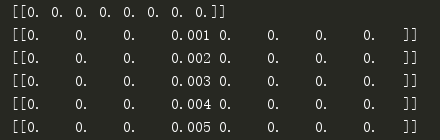
中间省略
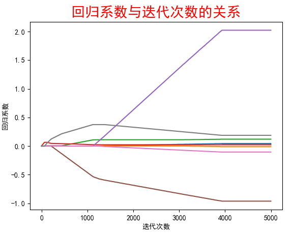
当迭代次数很大时,接近于普通最小二乘回归
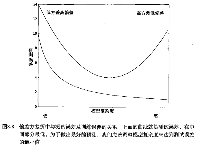
小结:当使用缩减方法时,把一些系数的回归系数缩减到0,减少了模型的复杂度,增加了模型的偏差,同时减小了方差
权衡偏差和方差
1.3 实例:预测乐高玩具价格
在交叉验证中使用90%数据集作为训练数据,10%做为测试数据,通过10次迭代之后,求30个不同lambda下的误差均值,再选择最小的误差,从而获取最优回归系数。
使用岭回归时需要对x数据集进行标准化,对y数据集进行中心化。最后需要对计算的回归系数进行还原,同时截距等于![]()
# encoding: utf-8
'''
@Author: shuhan Wei
@File: legao.py
@Time: 2018/8/24 16:16
'''
#BeautifulSoup是一个可以从HTML或XML文件中提取数据的Python库
import random

from bs4 import BeautifulSoup
import numpy as np
import regression
import ridgeRegression

def rssError(yArr,yHatArr): #yArr and yHatArr both need to be arrays
    return ((yArr-yHatArr)**2).sum()

def scrapePage(inFile, outFile, yr, numPce, origPrc):
    # 打开并读取HTML文件
    with open(inFile, encoding='utf-8') as fr:
        html = fr.read()
    fw = open(outFile, 'a')  # a是追加模式
    soup = BeautifulSoup(html)
    i = 1
    currentRow = soup.findAll('table', r="%d" % i)
    while (len(currentRow) != 0):
        currentRow = soup.findAll('table', r="%d" % i)
        title = currentRow[0].findAll('a')[1].text
        lwrTitle = title.lower()
        print(lwrTitle)
        if (lwrTitle.find('new') > -1) or (lwrTitle.find('nisb') > -1):
            newFlag = 1.0   #全新
        else:
            newFlag = 0.0   #不是全新
        soldUnicde = currentRow[0].findAll('td')[3].findAll('span')
        if len(soldUnicde) == 0:
            print
            "item #%d did not sell" % i
        else:
            soldPrice = currentRow[0].findAll('td')[4]
            priceStr = soldPrice.text
            priceStr = priceStr.replace('$', '')  # strips out $
            priceStr = priceStr.replace(',', '')  # strips out ,
            if len(soldPrice) > 1:
                priceStr = priceStr.replace('Free shipping', '')  # strips out Free Shipping
            print
            "%s\t%d\t%s" % (priceStr, newFlag, title)
            fw.write("%d\t%d\t%d\t%f\t%s\n" % (yr, numPce, newFlag, origPrc, priceStr))
        i += 1
        currentRow = soup.findAll('table', r="%d" % i)
    fw.close()


def setDataCollect():
    scrapePage('setHtml/lego8288.html', 'out.txt', 2006, 800, 49.99)    #2006年出品,部件数目800,原价49.99
    scrapePage('setHtml/lego10030.html', 'out.txt', 2002, 3096, 269.99)
    scrapePage('setHtml/lego10179.html', 'out.txt', 2007, 5195, 499.99)
    scrapePage('setHtml/lego10181.html', 'out.txt', 2007, 3428, 199.99)
    scrapePage('setHtml/lego10189.html', 'out.txt', 2008, 5922, 299.99)
    scrapePage('setHtml/lego10196.html', 'out.txt', 2009, 3263, 249.99)


"""
    函数说明:交叉验证测试岭回归
    Parameters:
        xArr - x数据集
        yArr - y数据集
        numVal - 交叉验证的次数
"""
def crossValidation(xArr,yArr,numVal=10):
    m = len(yArr)
    indexList = list(range(m))  #生成索引列表
    errorMat = np.zeros((numVal,30))#存放误差值
    for i in range(numVal):
        trainX=[]; trainY=[]
        testX = []; testY = []
        random.shuffle(indexList)    #打乱indexList,为了下面随机选取数据
        for j in range(m):  #使用90%的数据做训练集,10%做测试集
            if j < m * 0.9:
                trainX.append(xArr[indexList[j]])
                trainY.append(yArr[indexList[j]])
            else:
                testX.append(xArr[indexList[j]])
                testY.append(yArr[indexList[j]])
        wMat = ridgeRegression.ridgeTest(trainX,trainY)    #使用岭回归获取30组回归系数
        print(wMat)
        for k in range(30):#loop over all of the ridge estimates
            matTestX = np.mat(testX); matTrainX = np.mat(trainX)
            meanTrain = np.mean(matTrainX,0)
            varTrain = np.var(matTrainX,0)
            matTestX = (matTestX-meanTrain)/varTrain #正规化测试数据
            yEst = matTestX * np.mat(wMat[k,:]).T + np.mean(trainY)#计算预测y值
            errorMat[i,k] = rssError(yEst.T.A,np.array(testY))
            #print errorMat[i,k]
    meanErrors = np.mean(errorMat,0)#calc avg performance of the different ridge weight vectors
    minMean = float(min(meanErrors))    #获取最小的误差值
    bestWeights = wMat[np.nonzero(meanErrors==minMean)]
    #can unregularize to get model
    #when we regularized we wrote Xreg = (x-meanX)/var(x)
    #we can now write in terms of x not Xreg:  x*w/var(x) - meanX/var(x) +meanY
    xMat = np.mat(xArr); yMat = np.mat(yArr).T
    meanX = np.mean(xMat,0); varX = np.var(xMat,0)
    unReg = bestWeights / varX
    print("the best model from Ridge Regression is:\n",unReg)
    print("with constant term: ",-1*np.sum(np.multiply(meanX,unReg),1) + np.mean(yMat))  #常数项


if __name__ == '__main__':
    # setDataCollect()
    lgX, lgY = regression.loadDataSet('out.txt')
    #加上X0
    lgXMat = np.mat(np.ones((np.shape(lgX)[0],np.shape(lgX)[1]+1)))
    lgXMat[:,1:5] = np.mat(lgX)
    print(lgXMat[0])
    ws = regression.standRegres(lgXMat,lgY)
    print(ws)
    print(lgXMat[0]*ws,lgY[0])
    crossValidation(lgX,lgY)
使用最小二乘回归预测结果为:

它对数据拟合得很好,但看上去却没什么道理,从公式看零部件数量越多,反而销售价更低。
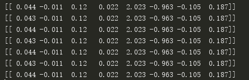
使用岭回归:
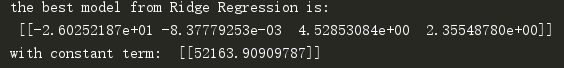

该结果和最小二乘结果没有太大差异,我们本期望找到一个更易于理解的模型,显然没有达到预期效果。为了达到这一点,我们看一下在缩减回归中系数是如何变化的

看运行结果的第一行,可以看到最大的是第4项,第二大的是第2项。因此,如果只选择一个特征来做预测的话,我们应该选择第4个特征,也就是原始加个。如果可以选择2个特征的话,应该选择第4个和第2个特征。
这种分析方法使得我们可以挖掘大量数据的内在规律。在仅有4个特征时,该方法的效果也许并不明显;但如果有100个以上的特征,该方法就会变得十分有效:它可以指出哪个特征是关键的,而哪些特征是不重要的。
使用sklearn中的岭回归
def usesklearn():
    from sklearn import linear_model
    reg = linear_model.Ridge(alpha=.5)
    lgX, lgY = regression.loadDataSet('out.txt')
    reg.fit(lgX, lgY)
    print("$%f%f*Year%f*NumPieces+%f*NewOrUsed+%f*original price" % (reg.intercept_, reg.coef_[0], reg.coef_[1], reg.coef_[2], reg.coef_[3],reg.coef[4]))
输出结果: