Contrastive Self-Supervised Learning

Contrastive Self-Supervised Learning

2020-01-30 10:32:24

 

Source: https://ankeshanand.com/blog/2020/01/26/contrative-self-supervised-learning.html 

 

Jan 26, 2020

Contrastive self-supervised learning techniques are a promising class of methods that build representations by learning to encode what makes two things similar or different.

The prophecy that self-supervised methods would replace the dominant direct supervision paradigm in deep learning has been around for quite some time. Alyosha Efros famously made a bet (the Gelato Bet) that an unsupervised method would beat a supervised R-CNN on Pascal VOC detection by Fall 2015. He would go on to lose the bet, but four years later, the prediction has been now been realized. Self-supervised methods now surpass their supervised counterparts at Pascal VOC detection (MoCo, He et al., 2019) and have shown great results at a lot of other tasks. The family of methods that have been behind this recent resurgence of self-supervised learning follow a paradigm called contrastive learning.

---

A large class of contemporary ML methods rely on human provided-labels or rewards as the only form of learning signal used during the training process. This over-reliance on direct-semantic supervision has several perils:

• The underlying data has a much richer structure than what sparse labels or rewards could provide. Thus, purely supervised learning algorithms often require large numbers of samples to learn from, and converge to brittle solutions.
• We can’t rely on direct supervision in high dimensional problems, and the marginal cost of acquiring labels is higher in problems like RL.
• It leads to task-specific solutions, rather than knowledge that can be repurposed.

Self-Supervised Learning provides a promising alternative, where the data itself provides the supervision for a learning algorithm. In this post, I will try to give an overview of how contrastive methods differ from other self-supervised learning techniques, and go over some of the recent papers in this area.

An illustrative example

 

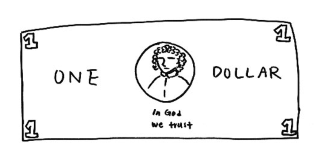
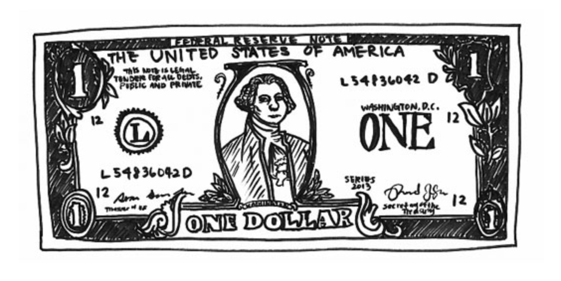
Fig. Left: Drawing of a dollar bill from memory. Right: Drawing subsequently made with a dollar bill present. Image source: Epstein, 2016

Consider this experiment conducted by Epstein, 2016 where subjects were asked to draw a picture of the dollar bill as detailed as possible.

Figure on the left shows the drawing a subject made by recalling what a dollar bill looks like from memory. Figure on the right is their drawing subsequently made with a dollar bill present. As is evident, the drawing made in the absence of the dollar bill is quite different compared with the drawing made from an exemplar.

Despite having seen a dollar bill countless number of times, we don’t retain a full representation of it. In fact, we really only retain enough features of the bill to distinguish it from other objects Similarly, can we build representation learning algorithms that don’t concentrate on pixel-level details, and only encode high-level features sufficient enough to distinguish different objects?

Generative vs Contrastive Methods

Contemporary self-supervised learning methods can roughly be broken down into two classes of methods:

Generative / Predictive

 Loss measured in the output space
Examples: Colorization, Auto-Encoders

 

Contrastive

 Loss measured in the representation space
Examples: TCN, CPC, Deep-InfoMax

 

Contrastive methods, as the name implies, learn representations by contrasting positive and negative examples. Although not a new paradigm, they have led to great empirical success in computer vision tasks with unsupervised contrastive pre-training.

Most notably:

• Contrastive methods trained on unlabelled ImageNet data and evaluated with a linear classifier now surpass the accuracy of supervised AlexNet. They also exhibit significant data efficiency when learning from labelled data compared to purely supervised learning (Data-Efficient CPC, Hénaff et al., 2019).
• Contrastive pre-training on ImageNet successfully transfers to other downstream tasks and outperforms the supervised pre-training counterparts (MoCo, He et al., 2019).

They differ from the more traditional generative methods to learn representations, which focus on reconstruction error in the pixel space to learn representations.

• Using pixel-level losses can lead to such methods being overly focused on pixel-based details, rather than more abstract latent factors.
• Pixel-based objectives often assume independence between each pixel, thereby reducing their ability to model correlations or complex structure.

How do contrastive methods work?

More formally, for any data point xx, contrastive methods aim to learn an encoder ff such that:

• here x+x+ is data point similar or congruent to xx, referred to as a positive sample.
• x−x− is a data point dissimilar to xx, referred to as a negative sample.
• the scorescore function is a metric that measures the similarity between two features.

xx is commonly referred to as an “anchor” data point. To optimize for this property, we can construct a softmax classifier that classifies positive and negative samples correctly. This should encourage the score function to assign large values to positive examples and small values to negative examples:

The denominator terms consist of one positive, and N−1N−1 negative samples. Here, we have used the dot product as the score function:

score(f(x),f(x+))=f(x)Tf(x+)score(f(x),f(x+))=f(x)Tf(x+)

This is the familiar cross-entropy loss for an NN-way softmax classifier, and commonly called the InfoNCE loss in the contrastive learning literature. It has been referred to as multi-class n-pair loss and ranking-based NCE in previous works.

The InfoNCE objective is also connected to mutual information. Specifically, minimizing the InfoNCE loss maximizes a lower bound on the mutual information between f(X)f(X) and f(X+)f(X+). See Poole et al., 2019 for a derivation and more details on this bound.

Let’s look at the different contrastive methods more closely to understand what they are doing:

Deep InfoMax

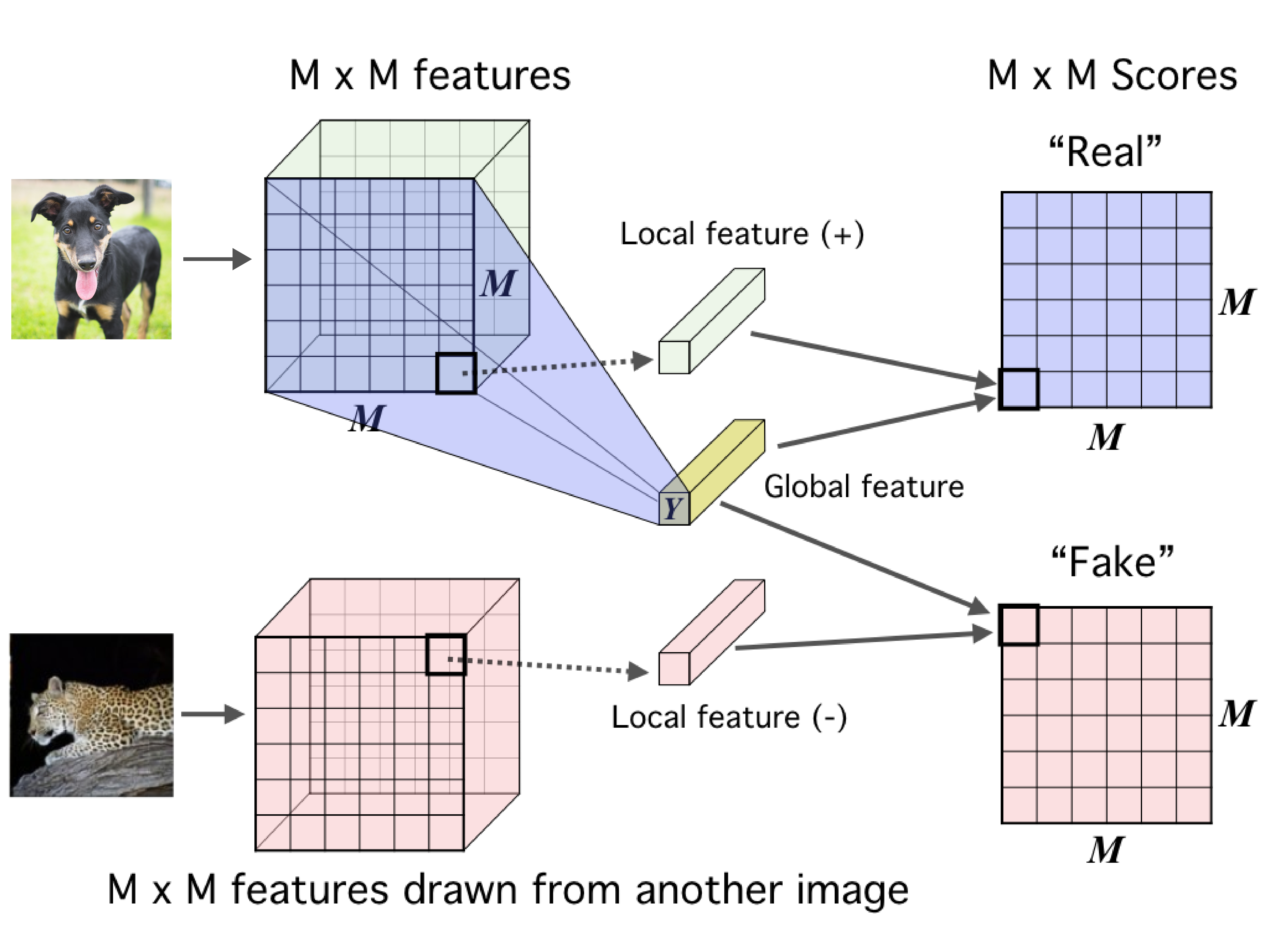
Fig.: The contrastive task in Deep InfoMax. Image source: Hjelm et al., 2018

Deep InfoMax (DIM, Hjelm et al., 2018) learns representations of images by leveraging the local structure present in an image. The contrastive task behind DIM is to classify whether a pair of global features and local features are from the same image or not. Here, global features are the final output of a convolutional encoder (a flat vector, Y) and local features are the output of an intermediate layer in the encoder (an M x M feature map). Each local feature map has a limited receptive field. So, intuitively this means to do well at the contrastive task the global feature vector must capture information from all the different local regions.

The loss function for DIM looks exactly as the contrastive loss function we described above. Given an anchor image x,

• f(x)f(x) refers to the global features.
• f(x+)f(x+) refers to the local features from the same image (positive samples).
• f(x−)f(x−) refers to the local features from a different image (negative samples).

DIM has been extended to other domains such as graphs (Veličković et al., 2018), and RL environments (Anand et al., 2019). A follow-up to DIM, Augment Multiscale DIM (Bachman et al., 2019) now achieves a 68.4% Top-1 accuracy on ImageNet with unsupervised training when evaluated with the linear classification protocol.

Contrastive Predictive Coding

Contrastive Predictive Coding (CPC, van den Oord et al., 2018) is a contrastive method that can be applied to any form of data that can be expressed in an ordered sequence: text, speech, video, even images (an image can be seen as a sequence of pixels or patches).

CPC learns representations by encoding information that’s shared across data points multiple time steps apart, discarding local information. These features are often called “slow features”: features that don’t change too quickly across time. Examples include identity of a speaker in an audio signal, an activity carried out in a video, an object in an image etc.

Fig.: Illustration of the contrastive task in CPC wih an audio input . Image adapted from van den Oord et al., 2018

The contrastive task in CPC is set as follows. Let {x1,x2,…,xN}{x1,x2,…,xN} be a sequence of data points, and xtxt be an anchor data point. Then,

• xt+kxt+k will be a positive sample for this anchor.
• A data point xt∗xt∗ randomly sampled from the sequence will be a negative sample.

CPC makes use of multiple kks in a single task to capture features evolving at different time scales.

When computing the representation for xtxt, we can use an autoregressive network that runs on top of the encoder network to encode the historical context.

Recent work (Hénaff et al., 2019) has scaled up CPC and achieved a 71.5 % top-1 accuracy when evaluated with linear classification on ImageNet.

Learning Invariances with Contrastive Learning

Fig. Left: AMDIM learns representations that are invariant across data augmentations such as random-crop. Right: CMC learns representations that are invariant across different views (channels) of an image. Image source: Bachman et al., 2019 and Tian et al., 2019

Contrastive Learning provides an easy way to impose invariances in the representation space. Suppose we want a representation to be invariant to a transformation TT (for example crops, grayscaling), we can simply construct a contrastive objective where given an anchor data point xx,

• T(x)T(x) is a positive sample
• T(x′)T(x′) where x′x′ is a random image or data point is a negative sample.

Several recent papers have used this and to great empirical successes:

• Augmented Multiscale DIM (AMDIM, Bachman et al., 2019) uses standard data augmentation techniques as the set of transformations a representation should be invariant to.
• Contrastive MultiView Coding (CMC, Tian et al., 2019) uses different views of the same image (depth, luminance, luminance, chrominance, surface normal, and semantic labels) as the set of transformations the representation should be invariant to.

Scaling the number of negative examples (MoCo)

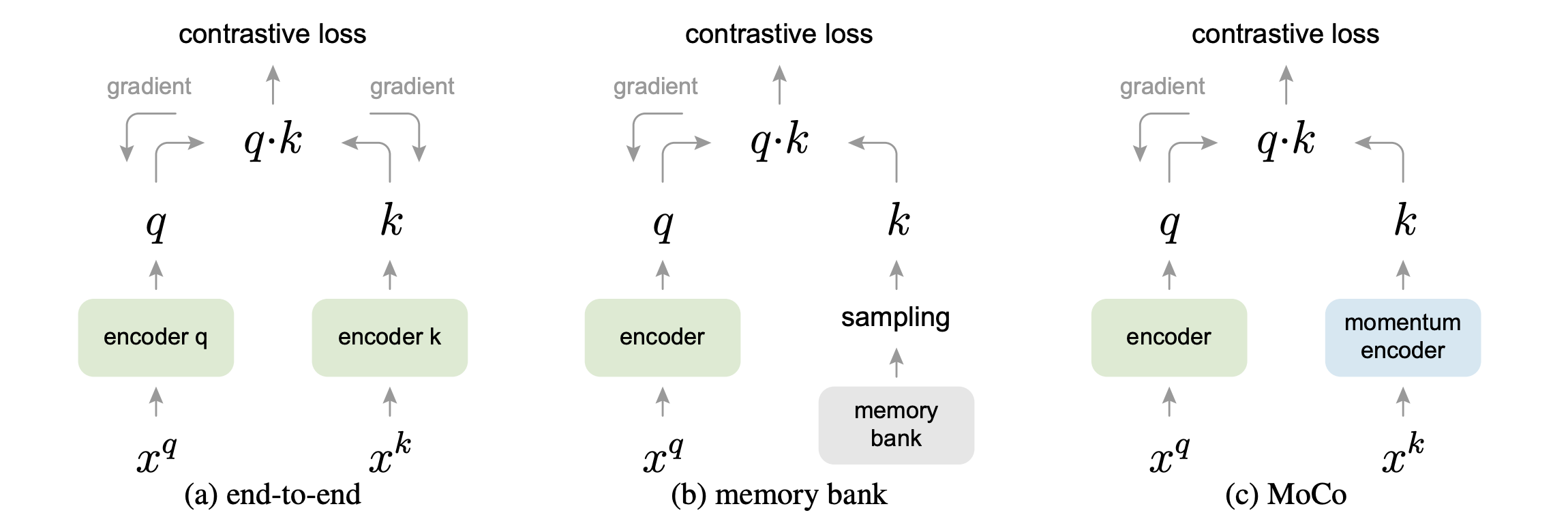
 Fig: Comparison of different strategies of using negative samples in contrastive methods. Here xqxq are positive examples, and xkxk are negative examples. Note that the gradient doesn’t flow back through the momentum encoder in MoCo. Image source: He et al., 2019

Contrastive methods tend to work better with more number of negative examples, since presumably larger number of negative examples may cover the underlying distribution more effectively and thus give a better training signal. In the usual formulation of contrastive learning, the gradients flow back through the encoders of both the positive and negative samples. This means that the number of negative samples is restricted to the size of the mini-batch. Momentum Contrast (MoCo, He et al., 2019) gets around this effectively by maintaining a large queue of negative samples, and not using backpropagation to update the negative encoder. Instead it periodically updates the negative encoder using a momentum update:

θk←mθk+(1−m)θqθk←mθk+(1−m)θq

Here, θkθk denotes the weights of the encoder for negative examples, and θqθq denotes the weights of the encoder for positive examples.

A pretty striking result from MoCo is that it can outperform its supervised pre-training counterpart in 7 detection/segmentation tasks on PASCAL VOC, COCO, and other datasets, sometimes surpassing it by large margins. Traditionally, these tasks needed supervised pre-training on ImageNet to achieve the best results, but MoCo’s results suggest that this gap between unsupervised and supervised pre-training has largely been closed.

A generic paradigm for self-supervised learning

Even though most applications of contrastive learning in this post have focused on standard computer vision tasks, I hope it’s evident contrastive learning is a domain and task agnostic paradigm for self-supervised learning. It allows us to inject our prior knowledge about the structure in the data into the representation space. This means that as we move away from static iid datasets (which discard a lot of underlying structure in the data) and leverage additional structural information, we can build more powerful self-supervised methods.

Acknowledgements

Thanks to Brady Neal, Evan Racah, Max Schwarzer and Sherjil Ozair for reviewing earlier drafts of this post and providing valuable feedback.

References

[1] Oord, Aaron van den, Yazhe Li, and Oriol Vinyals. “Representation learning with contrastive predictive coding.” “Representation Learning with Contrastive Predictive Coding” arXiv preprint arXiv:1807.03748, 2018.

[2] Hjelm, R. Devon, Alex Fedorov, Samuel Lavoie-Marchildon, Karan Grewal, Phil Bachman, Adam Trischler, and Yoshua Bengio. “Learning deep representations by mutual information estimation and maximization.” ICLR, 2019

[3] Sohn, Kihyuk. “Improved deep metric learning with multi-class n-pair loss objective.” NeurIPS, 2016.

[4] Hénaff, Olivier J., Ali Razavi, Carl Doersch, S. M. Eslami, and Aaron van den Oord. “Data-efficient image recognition with contrastive predictive coding.” arXiv preprint arXiv:1905.09272, 2019.

[5] He, Kaiming, Haoqi Fan, Yuxin Wu, Saining Xie, and Ross Girshick. “Momentum contrast for unsupervised visual representation learning.” arXiv preprint arXiv:1911.05722, 2019.

[6] Bachman, Philip, R. Devon Hjelm, and William Buchwalter. “Learning representations by maximizing mutual information across views.” NeurIPS, 2019.

[7] Tian, Yonglong, Dilip Krishnan, and Phillip Isola. “Contrastive multiview coding.” arXiv preprint arXiv:1906.05849, 2019.

[8] Veličković, Petar, William Fedus, William L. Hamilton, Pietro Liò, Yoshua Bengio, and R. Devon Hjelm. “Deep graph infomax.” ICLR, 2019.

[8] Anand, Ankesh, Evan Racah, Sherjil Ozair, Yoshua Bengio, Marc-Alexandre Côté, and R. Devon Hjelm. “Unsupervised state representation learning in atari.” NeurIPS, 2019.

[9] Sermanet, Pierre, Corey Lynch, Jasmine Hsu, and Sergey Levine. “Time-contrastive networks: Self-supervised learning from multi-view observation.” CVPRW, 2017.

[10] Poole, Ben, Sherjil Ozair, Aaron van den Oord, Alexander A. Alemi, and George Tucker. “On variational bounds of mutual information.” ICML, 2019.