机器学习- RNN以及LSTM的原理分析

• 概述

RNN是递归神经网络，它提供了一种解决深度学习的另一个思路，那就是每一步的输出不仅仅跟当前这一步的输入有关，而且还跟前面和后面的输入输出有关，尤其是在一些NLP的应用中，经常会用到，例如在NLP中，每一个输出的Word，都跟整个句子的内容都有关系，而不仅仅跟某一个词有关。LSTM是RNN的一种升级版本，它的核心思想跟RNN是一样的，但是它透过一下方法避免了一些RNN的缺点。那么下面就逐步的解析一下RNN和LSTM的结构，然后分析一下它们的原理吧。

• RNN解析

要理解RNN，咱们得先来看一下RNN的结构，然后就来解释一下它的原理

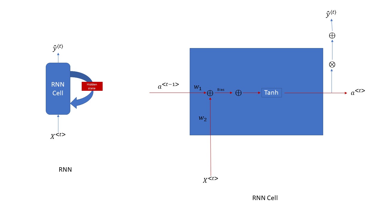
上图中左边的图是一个RNN网络结构中总体的图，右边的图片是一个RNN Cell里面的具体细节； 从上面的左边的图咱们可以看出，一个RNN的网络结构中，无论RNNcell循环多少次，它的weights都是share的，即一个weights只有一份copy， 而每一步的Hidden state(即右图中的a^<t>和a^<t-1>)是不同的，每一个time step它都有一份hidden state的copy。从上面的图片分析来看， RNN的每一步的输入不单单是有X^<t>, 而且还有有前面的time step中学习来的hidden state -  a^<t-1>。这就实现了咱们前面的需求了，让每一步的输出不仅仅跟当前的输入有关，还得跟前面的输入有关。具体的代码实现这个RNN cell的方法，你们可以参考下面的代码来加深对RNN的理解，实际在TensorFlow中来应用RNN的话，其实非常简单，就是一句代码就搞定了，但是，这里我还是贴出RNN cell创建的源码方便大家理解

def rnn_cell(xt, a_prev, parameters):
    """
    Implements a single forward step of the RNN-cell as described
    Arguments:
    xt -- your input data at timestep "t", numpy array of shape (n_x, m).
    a_prev -- Hidden state at timestep "t-1", numpy array of shape (n_a, m)
    parameters -- python dictionary containing:
                        Wax -- Weight matrix multiplying the input, numpy array of shape (n_a, n_x)
                        Waa -- Weight matrix multiplying the hidden state, numpy array of shape (n_a, n_a)
                        Wya -- Weight matrix relating the hidden-state to the output, numpy array of shape (n_y, n_a)
                        ba --  Bias, numpy array of shape (n_a, 1)
                        by -- Bias relating the hidden-state to the output, numpy array of shape (n_y, 1)
    Returns:
    a_next -- next hidden state, of shape (n_a, m)
    yt_pred -- prediction at timestep "t", numpy array of shape (n_y, m)
    cache -- tuple of values needed for the backward pass, contains (a_next, a_prev, xt, parameters)
    """
    
    # Retrieve parameters from "parameters"
    Wax = parameters["Wax"]
    Waa = parameters["Waa"]
    Wya = parameters["Wya"]
    ba = parameters["ba"]
    by = parameters["by"]

    # compute next activation state using the formula given above
    a_next = np.tanh(Wax.dot(xt)+Waa.dot(a_prev)+ba)
    # compute output of the current cell using the formula given above
    yt_pred = softmax(Wya.dot(a_next)+by)   
    
    # store values you need for backward propagation in cache
    cache = (a_next, a_prev, xt, parameters)
    
    return a_next, yt_pred, cache

np.random.seed(1)
xt_tmp = np.random.randn(3,10)
a_prev_tmp = np.random.randn(5,10)
parameters_tmp = {}
parameters_tmp['Waa'] = np.random.randn(5,5)
parameters_tmp['Wax'] = np.random.randn(5,3)
parameters_tmp['Wya'] = np.random.randn(2,5)
parameters_tmp['ba'] = np.random.randn(5,1)
parameters_tmp['by'] = np.random.randn(2,1)

a_next_tmp, yt_pred_tmp, cache_tmp = rnn_cell_forward(xt_tmp, a_prev_tmp, parameters_tmp)
print("a_next[4] = ", a_next_tmp[4])
print("a_next.shape = ", a_next_tmp.shape)
print("yt_pred[1] =", yt_pred_tmp[1])
print("yt_pred.shape = ", yt_pred_tmp.shape)
print( a_next_tmp[:,:])
print( a_next_tmp[:,0])

• LSTM解析

根据上面的RNN的结构图片，你们仔细的看一下有没有什么缺点。如果怎么的RNN需要循环很多次的话，咱们可能会有丢失信息的可能，就是gradient vanishing的情况发生，如果gradient vanishing的情况发生的话，它就不会继续学习咱们的信息了，就变成了standard neuro network了，RNN就失去了意义了。而且，咱们的sequence越长（即：循环的次数越多），gradient vanishing的可能性就越大。这个时候，咱们就有必要优化咱们的RNN了，让优化了的结构不但能够不断的学习能力，还能够有记忆功能，能把咱们学习的主要的东西能够记住，这就让咱们的RNN进化到了LSTM（Long short term memory）阶段了。为了能够更好的解释LSTM的网络结构，咱们还是先来看一些它就结构图片，然后再来解释一下吧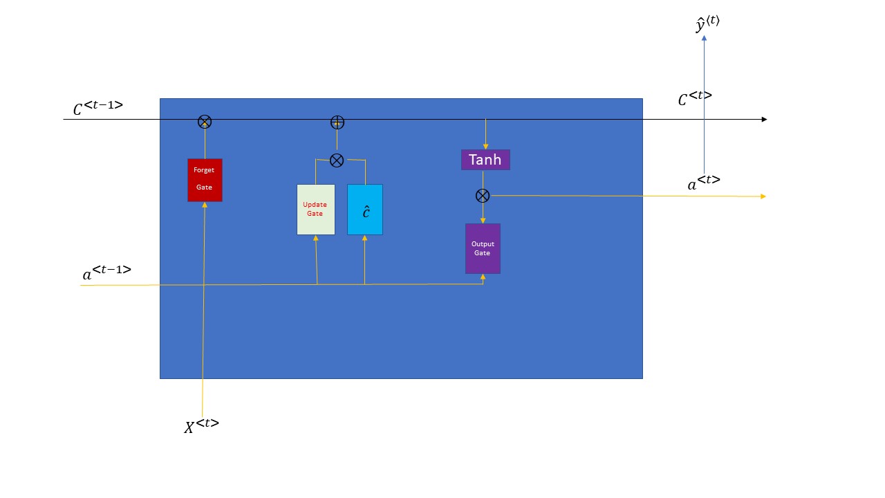

 上图是一个LSTM cell的基本结构，这个图有有些不重要的元素，我都省略了，主要留下了一些最重要的信息。首先对比RNN， 咱们可以看出咱们多了3个gate和一个memory cell - C^<t>。这个memory cell也称作internal hidden state。那么咱们来看看这个三个gate到底是干什么的。第一个gate是forget gate，它是帮助咱们的memory cell删除（或者称之为过滤）掉一些不重要的信息的，这个gate的值是在[0,1]这个区间，一般咱们用sigmoid函数来运算了，然后再和C来做element-wise的乘法运算，如果forget gate中的值趋向于0就删除掉相应的信息，如果forget gate中的值趋向于1则保留相应的值。第二个gate是update gate； 这个gate要跟咱们candidate memory cell来共同作用来产生新的信息，它们两个进行element-wise的相乘运算后，再跟咱们经过forget gate后的memory cell来进行element-wise的相加匀速，相当于把咱们从当前time step中学习到的信息添加到咱们的memory cell中。第三个gate就是output gate了；顾名思义就是过滤咱们输出的hidden state的, 这个gate也是sigmoid函数，根据前一个hidden state a^<t-1> 和当前time step的输入 X^<t>来共同决定的，它跟经过forget gate和update gate处理后的memory cell 的tanh值进行element-wise相乘过后，得到了了咱们当前time step的hidden state-a<t>，同时还得到了咱们当前time step的memory cell值；从这里咱们也可以看出output hidden state-a<t>和internal hidden state(memory cell）的dimension是一样的。上面解释了一下一个LSTM Cell中具体的结构跟功能。为了能够更好的加深大家对于LSTM的理解，我还是用代码演示一下如何构建一个LSTM cell， 代码如下所示：

 

def lstm_cell(xt, a_prev, c_prev, parameters):
    """
    Implement a single forward step of the LSTM-cell as described in Figure (4)

    Arguments:
    xt -- your input data at timestep "t", numpy array of shape (n_x, m).
    a_prev -- Hidden state at timestep "t-1", numpy array of shape (n_a, m)
    c_prev -- Memory state at timestep "t-1", numpy array of shape (n_a, m)
    parameters -- python dictionary containing:
                        Wf -- Weight matrix of the forget gate, numpy array of shape (n_a, n_a + n_x)
                        bf -- Bias of the forget gate, numpy array of shape (n_a, 1)
                        Wi -- Weight matrix of the update gate, numpy array of shape (n_a, n_a + n_x)
                        bi -- Bias of the update gate, numpy array of shape (n_a, 1)
                        Wc -- Weight matrix of the first "tanh", numpy array of shape (n_a, n_a + n_x)
                        bc --  Bias of the first "tanh", numpy array of shape (n_a, 1)
                        Wo -- Weight matrix of the output gate, numpy array of shape (n_a, n_a + n_x)
                        bo --  Bias of the output gate, numpy array of shape (n_a, 1)
                        Wy -- Weight matrix relating the hidden-state to the output, numpy array of shape (n_y, n_a)
                        by -- Bias relating the hidden-state to the output, numpy array of shape (n_y, 1)
                        
    Returns:
    a_next -- next hidden state, of shape (n_a, m)
    c_next -- next memory state, of shape (n_a, m)
    yt_pred -- prediction at timestep "t", numpy array of shape (n_y, m)
    cache -- tuple of values needed for the backward pass, contains (a_next, c_next, a_prev, c_prev, xt, parameters)
    
    Note: ft/it/ot stand for the forget/update/output gates, cct stands for the candidate value (c tilde),
          c stands for the cell state (memory)
    """

    # Retrieve parameters from "parameters"
    Wf = parameters["Wf"] # forget gate weight
    bf = parameters["bf"]
    Wi = parameters["Wi"] # update gate weight (notice the variable name)
    bi = parameters["bi"] # (notice the variable name)
    Wc = parameters["Wc"] # candidate value weight
    bc = parameters["bc"]
    Wo = parameters["Wo"] # output gate weight
    bo = parameters["bo"]
    Wy = parameters["Wy"] # prediction weight
    by = parameters["by"]
    
    # Retrieve dimensions from shapes of xt and Wy
    n_x, m = xt.shape
    n_y, n_a = Wy.shape

    ### START CODE HERE ###
    # Concatenate a_prev and xt 
    concat = np.concatenate((a_prev, xt), axis=0)

    # Compute values for ft (forget gate), it (update gate),
    # cct (candidate value), c_next (cell state), 
    # ot (output gate), a_next (hidden state)
    ft = sigmoid(Wf.dot(concat)+bf)        # forget gate
    it = sigmoid(Wi.dot(concat)+bi)        # update gate
    cct = np.tanh(Wc.dot(concat)+bc)       # candidate value
    c_next = c_prev*ft + cct*it   # cell state
    ot = sigmoid(Wo.dot(concat)+bo)        # output gate
    a_next = ot*np.tanh(c_next)    # hidden state
    
    # Compute prediction of the LSTM cell
    yt_pred = softmax(Wy.dot(a_next)+by)    
    ### END CODE HERE ###

    # store values needed for backward propagation in cache
    cache = (a_next, c_next, a_prev, c_prev, ft, it, cct, ot, xt, parameters)

    return a_next, c_next, yt_pred, cache

np.random.seed(1)
xt_tmp = np.random.randn(3,10)
a_prev_tmp = np.random.randn(5,10)
c_prev_tmp = np.random.randn(5,10)
parameters_tmp = {}
parameters_tmp['Wf'] = np.random.randn(5, 5+3)
parameters_tmp['bf'] = np.random.randn(5,1)
parameters_tmp['Wi'] = np.random.randn(5, 5+3)
parameters_tmp['bi'] = np.random.randn(5,1)
parameters_tmp['Wo'] = np.random.randn(5, 5+3)
parameters_tmp['bo'] = np.random.randn(5,1)
parameters_tmp['Wc'] = np.random.randn(5, 5+3)
parameters_tmp['bc'] = np.random.randn(5,1)
parameters_tmp['Wy'] = np.random.randn(2,5)
parameters_tmp['by'] = np.random.randn(2,1)

a_next_tmp, c_next_tmp, yt_tmp, cache_tmp = lstm_cell_forward(xt_tmp, a_prev_tmp, c_prev_tmp, parameters_tmp)
print("a_next[4] = 
", a_next_tmp[4])
print("a_next.shape = ", c_next_tmp.shape)
print("c_next[2] = 
", c_next_tmp[2])
print("c_next.shape = ", c_next_tmp.shape)
print("yt[1] =", yt_tmp[1])
print("yt.shape = ", yt_tmp.shape)
print("cache[1][3] =
", cache_tmp[1][3])
print("len(cache) = ", len(cache_tmp))

• 总结

上面的两个部分主要介绍了RNN和LSTM的结构，以及分析了它们结构内部的功能和流程。并且分别在每一个cell后面都用Python展示了如何用代码去构建一个RNN cell和LSTM cell。咱们可以理解LSTM是对RNN的一种优化，同时要明白为什么要进行这样的优化；其次最重要的是理解RNN的这样一种新的解决问题的方法和思路，这跟咱们之前见过的standard neuro network最明显的一个区别就是，之前在神经网络，regressor 或者classfier中，每一个输出只跟咱们的输入features相关， 而RNN的思路则是不仅仅跟当前的输入有关，还跟前面的输入有关，这在以前sequence model中是非常常见的，例如Language modeling, machine translation等等的应用中，都是要用到RNN的思想的。