例子 gist 来自之前的 Trie 的实现, Ruby vs Go.

main 函数加上了下面几行:

1
2
3
4
5
6
import "runtime/pprof"
// ...
cpuProfile, _ := os.Create("cpu_profile")
pprof.StartCPUProfile(cpuProfile)
defer pprof.StopCPUProfile()
// ...

这里 os.Create("cpu_profile") 指定生成的数据文件, 然后 pprof.StartCPUProfile 看名字就知道是开始对 CPU 的使用进行监控. 有开始就有结束, 一般直接跟着 defer pprof.StopCPUProfile() 省的后面忘了. 编译执行一次以后会在目录下生成监控数据并记录到 cpu_profile. 接着就可以使用 pprof 来解读分析这些监控生成的数据.

When CPU profiling is enabled, the Go program stops about 100 times per second and records a sample consisting of the program counters on the currently executing goroutine’s stack.

CPU Profiling

1
2
3
4
5
6
$ go tool pprof cpu_profile
Type: cpu
Time: Jan 22, 2019 at 3:02pm (CST)
Duration: 518.52ms, Total samples = 570ms (109.93%)
Entering interactive mode (type "help" for commands, "o" for options)
(pprof)

因为是在多核环境, 所以, 取样时间(Total samples) 占比大于 100% 也属于正常的. 交互操作模式提供了一大票的命令, 执行一下 help 就有相应的文档了. 比如输出报告到各种格式(pdf, png, gif), 方块越大个表示消耗越大.

又或者列出 CPU 占比最高的一些(默认十个)运行结点的 top 命令, 也可以加上需要的结点数比如 top15

 1
 2
 3
 4
 5
 6
 7
 8
 9
10
11
12
13
14
(pprof) top
Showing nodes accounting for 480ms, 84.21% of 570ms total
Showing top 10 nodes out of 67
    flat  flat%   sum%        cum   cum%
    200ms 35.09% 35.09%      210ms 36.84%  main.NewNode (inline)
    70ms 12.28% 47.37%      170ms 29.82%  runtime.scanobject
    60ms 10.53% 57.89%       70ms 12.28%  runtime.greyobject
    30ms  5.26% 63.16%       30ms  5.26%  runtime.memclrNoHeapPointers
    30ms  5.26% 68.42%       30ms  5.26%  runtime.memmove
    20ms  3.51% 71.93%      250ms 43.86%  main.(*Node).insert
    20ms  3.51% 75.44%       20ms  3.51%  runtime.findObject
    20ms  3.51% 78.95%      230ms 40.35%  runtime.gcDrain
    20ms  3.51% 82.46%       20ms  3.51%  runtime.pthread_cond_wait
    10ms  1.75% 84.21%       10ms  1.75%  runtime.(*gcWork).tryGetFast (inline)
  • flat: 是指该函数执行耗时, 程序总耗时 570ms, main.NewNode 的 200ms 占了 35.09%
  • sum: 当前函数与排在它上面的其他函数的 flat 占比总和, 比如 35.09% + 12.28% = 47.37%
  • cum: 是指该函数加上在该函数调用之前累计的总耗时, 这个看图片格式的话会更清晰一些.

可以看到, 这里最耗 CPU 时间的是 main.NewNode 这个操作.

除此外还有 list 命令可以根据匹配的参数列出指定的函数相关数据, 比如:

Memory Profiling

1
2
3
// ...
memProfile, _ := os.Create("mem_profile")
pprof.WriteHeapProfile(memProfile)

类似 CPU 的监控, 要监控内存的分配回收使用情况, 只要调用 pprof.WriteHeapProfile(memProfile)

然后是跟上面一样的生成图片:

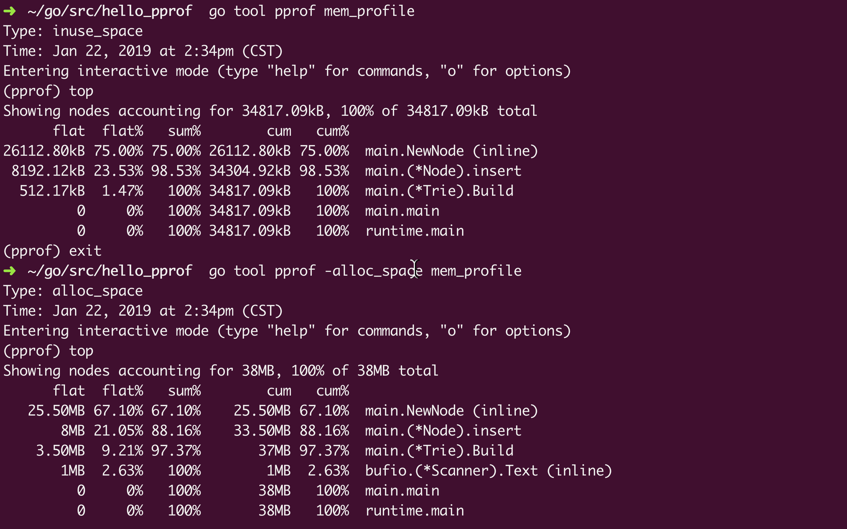
Type: inuse_space 是监控内存的默认选项, 还可以选 -alloc_space, -inuse_objects, -alloc_objects

inuse_space 是正在使用的内存大小, alloc_space是从头到尾一共分配了的内存大小(包括已经回收了的), 后缀为 _objects 的是相应的对象数

net/http/pprof

对于 http 服务的监控有一些些的不同, 不过 Go 已经对 pprof 做了一些封装在 net/http/pprof

例子 gist 来自从 net/http 入门到 Gin 源码梳理

引入多一行 _ "net/http/pprof", 启用服务以后就可以在路径 /debug/pprof/ 看到相应的监控数据. 类似下面(已经很贴心的把各自的描述信息写在下边了):

用 wrk (brew install wrk) 模拟测试

wrk -c 200 -t 4 -d 3m http://localhost:8080/hello

还是没有前面的那些可视化图形 UI 直观, 不过可以通过 http://localhost:8080/debug/pprof/profile (其他几个指标也差不多, heap, alloc…)生成一个类似前面的 CPU profile 文件监控 30s 内的数据. 然后就可以用 go tool pprof来解读了.

 1
 2
 3
 4
 5
 6
 7
 8
 9
10
11
12
13
14
15
16
17
18
19
20
21
22
23
24
25
26
27
28
29
30
31
32
33
34
35
36
37
38
39
40
Type: cpu
Time: Jan 22, 2019 at 4:22pm (CST)
Duration: 30.13s, Total samples = 1.62mins (321.66%)
Entering interactive mode (type "help" for commands, "o" for options)
(pprof) top
Showing nodes accounting for 93.78s, 96.76% of 96.92s total
Dropped 270 nodes (cum <= 0.48s)
Showing top 10 nodes out of 52
      flat  flat%   sum%        cum   cum%
    81.42s 84.01% 84.01%     81.45s 84.04%  syscall.Syscall
     3.45s  3.56% 87.57%      3.45s  3.56%  runtime.kevent
     2.31s  2.38% 89.95%      2.31s  2.38%  runtime.pthread_cond_wait
     2.06s  2.13% 92.08%      2.07s  2.14%  runtime.usleep
     1.93s  1.99% 94.07%      1.93s  1.99%  runtime.pthread_cond_signal
     1.10s  1.13% 95.20%      1.10s  1.13%  runtime.freedefer
     0.85s  0.88% 96.08%      0.87s   0.9%  runtime.nanotime
     0.59s  0.61% 96.69%      4.07s  4.20%  runtime.netpoll
     0.04s 0.041% 96.73%      0.67s  0.69%  runtime.newproc1
     0.03s 0.031% 96.76%     44.18s 45.58%  net/http.(*conn).readRequest
(pprof)

Type: alloc_space
Time: Jan 22, 2019 at 4:26pm (CST)
Entering interactive mode (type "help" for commands, "o" for options)
(pprof) top
Showing nodes accounting for 21.91GB, 99.82% of 21.95GB total
Dropped 66 nodes (cum <= 0.11GB)
Showing top 10 nodes out of 16
      flat  flat%   sum%        cum   cum%
    6.72GB 30.61% 30.61%     6.72GB 30.62%  net/textproto.(*Reader).ReadMIMEHeader
    5.97GB 27.18% 57.80%    20.54GB 93.60%  net/http.(*conn).readRequest
       4GB 18.21% 76.01%    13.23GB 60.30%  net/http.readRequest
    2.01GB  9.16% 85.17%     2.01GB  9.16%  net/url.parse
    1.25GB  5.71% 90.88%     1.25GB  5.71%  net.(*conn).Read
    1.22GB  5.54% 96.42%     1.22GB  5.55%  context.WithCancel
    0.49GB  2.25% 98.68%     0.49GB  2.25%  net/textproto.(*Reader).ReadLine
    0.13GB  0.58% 99.25%     0.13GB  0.58%  main.main.func1
    0.12GB  0.56% 99.82%     0.12GB  0.56%  bufio.NewWriterSize (inline)
         0     0% 99.82%     0.13GB  0.59%  net/http.(*ServeMux).ServeHTTP
(pprof)

gin pprof

import _ "net/http/pprof" 实际上是为了执行包 net/http/pprof 中的 init 函数.

1
2
3
4
5
6
7
8
// pprof.go
func init() {
    http.HandleFunc("/debug/pprof/", Index)
    http.HandleFunc("/debug/pprof/cmdline", Cmdline)
    http.HandleFunc("/debug/pprof/profile", Profile)
    http.HandleFunc("/debug/pprof/symbol", Symbol)
    http.HandleFunc("/debug/pprof/trace", Trace)
}

因此, Gin 项目要使用 pprof 的话可以参考这里

Flame Graph 火焰图

go-torch 在 Go 1.11 之前是作为非官方的可视化工具存在的, 它可以为监控数据生成一个类似下面这样的图形界面, 红红火火的, 因而得名. 从 Go 1.11 开始, 火焰图被集成进入 Go 官方的 pprof 库.

go-torch is deprecated, use pprof instead

As of Go 1.11, flamegraph visualizations are available in go tool pprof directly!

1
$ go tool pprof -http=":8081" [binary] [profile]

在浏览器打开 http://localhost:8081/ui/flamegraph, 就可以看到下面这样的反过来的火焰图.

长条形的颜色只是为了好看, 颜色的深浅是随机的 = 。= 长度越长代表占用 CPU 时间越长

然后, pprof 命令行的 top 以及 list 正则也可以在这里边完成, 还有 svg 图形.

基于Chrome的图形trace/debug

Trace概览

让我们从一个简单的“Hello,world”示例开始。在本例中,我们使用runtime/trace包将trace数据写入标准错误输出。

package main

import (    
   "os"    "runtime/trace"
)

func main() {    trace.Start(os.Stderr)    
   defer trace.Stop()    
   // create new channel of type int    ch := make(chan int)    
   
   // start new anonymous goroutine    go func() {        
       // send 42 to channel        ch <- 42    }()    
   // read from channel    <-ch }

这个例子创建了一个无缓冲的channel,初始化一个goroutine,并发送数字42到channel。运行主goroutine时是阻塞的,它会等待另一个goroutines发送一个int数值给channel。

用 go run main.go 2> trace.out 运行这段代码会发送trace数据到trace.out,之后可以用 go tool trace trace.out 读取trace。(该程序是个web app,默认启动127.0.0.1地址的一个随机端口,如果需要修改host可以加参数解决,例如 go tool trace --http=':8080' trace.out,译者加)  

Tips: go 1.8之前,你同时需要可执行二进制文件和trace数据来分析trace;用go 1.8之后的版本编译的程序,trace数据已经包含了go tool trace命令所有的信息。
运行该命令后,在浏览器窗口打开该地址,它会提供一些选项。每一个都会打开trace的不同视图,涵盖了程序执行的不同信息。

1 View trace  

最复杂、最强大和交互式的可视化显示了整个程序执行的时间轴。这个视图显示了在每个虚拟处理器上运行着什么,以及什么是被阻塞等待运行的。稍后我们将在这篇文章中深入探讨这个视图。注意它只能在chrome上显示。

2 Goroutine analysis  

显示了在整个执行过程中,每种类型的goroutines是如何创建的。在选择一种类型之后就可以看到关于这种类型的goroutine的信息。例如,在试图从mutex获取锁、从网络读取、运行等等每个goroutine被阻塞的时间。

3 Network/Sync/Syscall blocking profile  

这些图表显示了goroutines在这些资源上所花费的时间。它们非常接近pprof上的内存/cpu分析。这是分析锁竞争的最佳选择。

4 Scheduler latency profiler  

为调度器级别的信息提供计时功能,显示调度在哪里最耗费时间。

View Trace

点击“View Trace”链接,你会看到一个界面,里面充满了关于整个程序执行的信息。Tips: 右上角的"?"按钮可以获取快捷方式列表,以帮助跟踪trace。
下面的图片突出了最重要的部分,图片下面是对每个部分的说明描述:

1 Timeline  

显示执行的时间,根据跟踪定位的不同,时间单位可能会发生变化。你可以通过使用键盘快捷键(WASD键,就像视频游戏一样)来导航时间轴。

2 Heap  

在执行期间显示内存分配,这对于发现内存泄漏非常有用,并检查垃圾回收在每次运行时能够释放多少内存。

3 Goroutines  

在每个时间点显示有多少goroutines在运行,有多少是可运行的(等待被调度的)。大量可运行的goroutines可能显示调度竞争,例如,当程序创建过多的goroutines,会导致调度程序繁忙。

4 OS Threads  

显示有多少OS线程正在被使用,有多少个被syscalls阻塞。

5 Virtual Processors  

每个虚拟处理器显示一行。虚拟处理器的数量由GOMAXPROCS环境变量控制(默认为内核数)。

6 Goroutines and events  

显示在每个虚拟处理器上有什么goroutine在运行。连接goroutines的连线代表事件。在示例图片中,我们可以看到goroutine "G1.runtime.main"衍生出了两个不同的goroutines:G6和G5(前者是负责收集trace数据的goroutine,后者是我们使用“go”关键字启动的那个)。每个处理器的第二行可能显示额外的事件,比如syscalls和运行时事件。这还包括goroutine代表运行时所做的一些工作(例如辅助垃圾回收)。下图显示了当选择一个goroutine时得到的信息。

该信息包含:

  •     它的“名称”(Title)

  •     何时开始(Start)

  •     持续时间(Wall Duration)

  •     开始时的栈trace

  •     结束时的栈trace

  •     该goroutine产生的事件

我们可以看到,这个goroutine创造了两个事件:

trace goroutine和在channel上发送42的goroutine。

通过点击一个特定的事件(点击图中的一条连线或者在点击goroutine后选择事件),我们可以看到:

  • 事件开始时的栈信息

  • 事件持续时长

  • 事件包含的goroutine

你可以点击这些goroutines来定位跟踪到它们的trace数据。

阻塞概况 

从trace中获得的另一个特殊视图是网络/同步/syscall阻塞概况。阻塞概况显示了一个类似于pprof的内存/cpu概况中的图形视图。不同之处在于,这些概况显示每个goroutine在一个特定资源上花费的阻塞时间,而不是显示每个函数分配了多少内存。下图告诉我们示例代码的“同步阻塞概况”

这告诉我们,我们的主goroutine从一个channel接收花费了12.08微秒。当太多的goroutines在竞争着获取一个资源的锁时,这种类型的图是找到锁竞争的很好的方法。

收集trace

有三种收集trace的方法:

1 使用 runtime/trace包  

这个需要调用trace.Starttrace.Stop,已经在我们的示例程序中讲过。

2 使用 -trace=<file>测试标志  

用来收集关于被测试代码的trace时比较有用。

3 使用 debug/pprof/tracehandler  

这是用来收集运行中的web应用的trace的最好的方法。

跟踪一个web应用


想要从一个运行的web应用收集trace, 你需要添加 /debug/pprof/trace handler。下面的代码示例展示了如何通过简单地导入 net/http/pprof 包为 http.DefaultServerMux 做到这一点。

package main

import (    
   "net/http"    _
   "net/http/pprof"
)

func main() {    http.Handle("/hello", http.HandlerFunc(helloHandler))    http.ListenAndServe("localhost:8181", http.DefaultServeMux) }

func helloHandler(w http.ResponseWriter, r *http.Request) {    w.Write([]byte("hello world!")) }


为了收集trace,我们需要向endpoint发出请求,例如,curl localhost:8181/debug/pprof/trace?seconds=10 > trace.out 此请求将阻塞10秒钟,trace数据将写入文件trace.out。像这样生成的trace可以像我们以前那样查看:go tool trace trace.out
Tips: 请注意,将pprof handlers暴露给Internet是不建议的。推荐的做法是在不同的只绑定到loopback接口的http.Server暴露这些endpoint。这篇博客(https://mmcloughlin.com/posts/your-pprof-is-showing)讨论该风险,并有代码示例解释如何正确地暴露pprof handler。

在收集trace之前,让我们首先通过wrk来给我们的服务加一些负载:$ wrk -c 100 -t 10 -d 60s http://localhost:8181/hello

这将使用10个线程的100个连接在60秒内发出请求。当wrk正在运行时,我们可以使用 curl localhost:8181/debug/pprof/trace?seconds=5 > trace.out 来收集5s的trace数据。这会产生一个5MB的文件(如果我们能够在我的4核CPU机器上生成更多的负载,它就可以快速增长)。同样,打开trace是由go tool trace命令完成的。当该工具解析文件的整个内容时,这将花费比我们之前的示例花费的时间更长。当它完成时,页面看起来略有不同:

View trace (0s-2.546634537s)
View trace (2.546634537s-5.00392737s)

Goroutine analysis
Network blocking profile
Synchronization blocking profile
Syscall blocking profile
Scheduler latency profile


为了保证浏览器渲染呈现所有内容,该工具将trace分为两个连续的部分。更复杂的应用或更长的trace可能需要工具将其分割成更多的部分。点击“View trace(2.546634537-5.00392737)”我们可以看到有很多事情正在发生:

这个特殊的屏幕截图显示了一个GC运行情况,它从1169ms-1170ms开始,在1174ms之后结束。在这段时间里,一个OS线程(PROC 1)运行一个用于GC的goroutine,而其他goroutines则在一些GC阶段中提供辅助(这些步骤显示在goroutine的连线中,并被叫做MARK ASSIST)。在截图的最后,我们可以看到大部分分配的内存都被GC释放了。  另一个特别有用的信息是在“Runnable”状态下的goroutines的数量(在选定的时间内是13):如果这个数字随着时间的推移变得很大,这就意味着我们需要更多的cpu来处理负载。


结论


trace程序是调试并发问题的强大工具。例如,竞争和逻辑冲突。但它并不能解决所有的问题:它并不是用来跟踪哪块代码花费最多CPU时间或分配的最佳工具。go tool pprof 更适用于这些用例。当你想要了解一个耗时程序的行为,并且想知道当每个goroutine不运行时它在做什么,这个工具就会很好地发挥作用。收集trace可能会有一些开销,并且会生成大量的数据用来检查。不幸的是,官方文档是缺失的,因此需要进行一些试验来尝试和理解trace程序所显示的内容。这也是对官方文档和整个社区作出贡献的机会(e.g 博客文章)。

参考 

Go execution tracer (design doc)

Using the go tracer to speed fractal rendering

Go tool trace

Your pprof is showing