第五周作业：卷积神经网络（Part3）

1、MobileNet

　　随着对准确度的要求越来越高，网络也越来越深。因此既能保持模型性能（accuracy）也能降低模型大小（parameters size）、同时提升模型速度（speed, low latency）的MobileNet应运而生。

　　MobileNet的基本单元是深度可分离卷积（depthwise separable convolution），包括深度卷积（depthwise convolution）和点卷积（pointwise convolution）。传统卷积分成两步，每个卷积核与每张特征图进行按位相乘然后进行相加，计算量为D_F∗D_F∗D_K∗D_K∗M∗N，其中D_F为特征图尺寸，D_K为卷积核尺寸，M为输入通道数，N为输出通道数。而深度可分离卷积首先对应不同的通道使用不同的卷积核，进行按位相乘的计算，通道数不变；然后使用1*1的卷积核进行传统的卷积运算，此时通道数可以进行改变，其计算量为D_K∗D_K∗M∗D_F∗D_F+1∗1∗M∗N∗D_F∗D_F。

　　

　　标准卷积和深度可分离卷积的基本结构如下所示，深度可分离卷积在深度卷积和点卷积后都应用了batchnorm和relu。

 　　

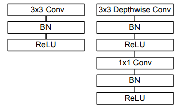
class Block(nn.Module):
    '''Depthwise conv + Pointwise conv'''
    def __init__(self, in_planes, out_planes, stride=1):
        super(Block, self).__init__()
        # Depthwise 卷积，3*3 的卷积核，分为 in_planes，即各层单独进行卷积
        self.conv1 = nn.Conv2d(in_planes, in_planes, kernel_size=3, stride=stride, padding=1, groups=in_planes, bias=False)
        self.bn1 = nn.BatchNorm2d(in_planes)
        # Pointwise 卷积，1*1 的卷积核
        self.conv2 = nn.Conv2d(in_planes, out_planes, kernel_size=1, stride=1, padding=0, bias=False)
        self.bn2 = nn.BatchNorm2d(out_planes)

    def forward(self, x):
        out = F.relu(self.bn1(self.conv1(x)))
        out = F.relu(self.bn2(self.conv2(out)))
        return out

　　

2、MobileNetV2

　　V2在V1的基础上，引入了Inverted Residuals和Linear Bottlenecks。

　　倒残差模块Inverted Residuals：在3x3网络结构前利用1x1卷积升维，在3x3网络结构后利用1x1卷积降维，先进行扩张，再进行压缩。ResNet里用的是残差模块，整个过程是“压缩-卷积-扩张”。这样做的目的是减少3*3模块的计算量，提高残差模块的计算效率。倒残差模块整个过程是“扩张-卷积-压缩”。因为depthwise卷积不能改变通道数，因此特征提取受限于输入的通道数，所以先提升通道数。

 　   Linear Bottlenecks：为了避免Relu对低维特征的破坏，在最后一层不使用relu而使用线性激活函数，其它层仍然使用relu。

　　

class Block(nn.Module):
    '''expand + depthwise + pointwise'''
    def __init__(self, in_planes, out_planes, expansion, stride):
        super(Block, self).__init__()
        self.stride = stride
        # 通过 expansion 增大 feature map 的数量
        planes = expansion * in_planes
        self.conv1 = nn.Conv2d(in_planes, planes, kernel_size=1, stride=1, padding=0, bias=False)
        self.bn1 = nn.BatchNorm2d(planes)
        self.conv2 = nn.Conv2d(planes, planes, kernel_size=3, stride=stride, padding=1, groups=planes, bias=False)
        self.bn2 = nn.BatchNorm2d(planes)
        self.conv3 = nn.Conv2d(planes, out_planes, kernel_size=1, stride=1, padding=0, bias=False)
        self.bn3 = nn.BatchNorm2d(out_planes)

        # 步长为 1 时，如果 in 和 out 的 feature map 通道不同，用一个卷积改变通道数
        if stride == 1 and in_planes != out_planes:
            self.shortcut = nn.Sequential(
                nn.Conv2d(in_planes, out_planes, kernel_size=1, stride=1, padding=0, bias=False),
                nn.BatchNorm2d(out_planes))
        # 步长为 1 时，如果 in 和 out 的 feature map 通道相同，直接返回输入
        if stride == 1 and in_planes == out_planes:
            self.shortcut = nn.Sequential()

    def forward(self, x):
        out = F.relu(self.bn1(self.conv1(x)))
        out = F.relu(self.bn2(self.conv2(out)))
        out = self.bn3(self.conv3(out))
        # 步长为1，加 shortcut 操作
        if self.stride == 1:
            return out + self.shortcut(x)
        # 步长为2，直接输出
        else:
            return out

　　

3、HybridSN

　　HybirdSN的主要特点是采用了3-D-CNN与2-D-CNN相结合的方式，既降低了3-D-CNN的模型复杂度，又弥补了2-D-CNN无法提取光谱维度特征的缺点。

　　　　　

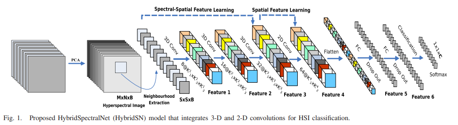
　　为了充分利用二维和三维cnn的特征自动学习能力，作者提出了HybridSN网络流程图如图所示，它包括三个三维卷积、一个二维卷积和三个完全连接的层。

• 三维卷积中，卷积核的尺寸为8×3×3×7×1、16×3×3×5×8、32×3×3×3×16（16个三维核，3×3×5维）
• 二维卷积中，卷积核的尺寸为64×3×3×576（576为二维输入特征图的数量）

　　三维卷积部分：

• conv1：（1, 30, 25, 25）， 8个 7x3x3 的卷积核 ==>（8, 24, 23, 23）
• conv2：（8, 24, 23, 23）， 16个 5x3x3 的卷积核 ==>（16, 20, 21, 21）
• conv3：（16, 20, 21, 21），32个 3x3x3 的卷积核 ==>（32, 18, 19, 19）

　　二维卷积：（576, 19, 19） 64个 3x3 的卷积核，得到 （64, 17, 17）

　　展平 flatten 操作，变为 18496 维的向量，接下来是256、128节点的全连接层，都使用比例为0.4的 Dropout，

　　最后输出为 16 个节点，是最终的分类类别数。 

class HybridSN(nn.Module):
  def __init__(self, num_classes=class_num):
    super(HybridSN,self).__init__()
    #先进行三维卷积
    #conv1：（1, 30, 25, 25）， 8个 7x3x3 的卷积核 ==>（8, 24, 23, 23）
    self.conv1 = nn.Conv3d(1, 8, kernel_size=(7,3,3), stride=1, padding=0, bias=False)
    self.bn1 = nn.BatchNorm3d(8)
    #self.layers = self._make_layers(in_planes=32)
    #conv2：（8, 24, 23, 23）， 16个 5x3x3 的卷积核 ==>（16, 20, 21, 21）
    self.conv2 = nn.Conv3d(8, 16, kernel_size=(5,3,3), stride=1, padding=0, bias=False)
    self.bn2 = nn.BatchNorm3d(16)
    #conv3：（16, 20, 21, 21），32个 3x3x3 的卷积核 ==>（32, 18, 19, 19）
    self.conv3 = nn.Conv3d(16, 32, kernel_size=(3,3,3), stride=1, padding=0, bias=False)
    self.bn3 = nn.BatchNorm3d(32)

    #二维卷积：（576, 19, 19） 64个 3x3 的卷积核，得到 （64, 17, 17）
    self.conv4 = nn.Conv2d(576, 64, kernel_size=(3,3), stride=1, padding=0)
    self.bn4 = nn.BatchNorm2d(64)
    #依次为256，128节点的全连接层，都使用比例为0.4的 Dropout
    self.fc1 = nn.Linear(18496,256)
    self.fc2 = nn.Linear(256,128)
    self.dropout = nn.Dropout(p = 0.4)
    self.fc3 = nn.Linear(128,num_classes)

  def forward(self, x):
    out = F.relu(self.bn1(self.conv1(x)))
    out = F.relu(self.bn2(self.conv2(out)))
    out = F.relu(self.bn3(self.conv3(out)))
    #进行二维卷积，因此把前面的 32*18 reshape 一下，得到 （576, 19, 19）
    out = out.reshape(out.shape[0],-1,19,19)
    out = F.relu(self.bn4(self.conv4(out)))
    #接下来是一个 flatten 操作，变为 18496 维的向量
    out = out.view(out.size(0), -1)
    out = F.relu(self.dropout(self.fc1(out)))
    out = F.relu(self.dropout(self.fc2(out)))
    out = F.relu(self.dropout(self.fc3(out)))
    return out

 　　

二、总结

　　这三篇之前看过也忘了，再看一遍温故知新。

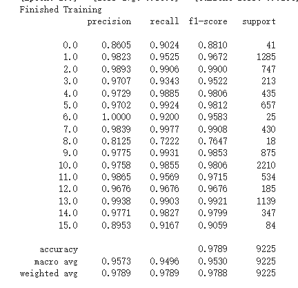
 　　对HybridSN网络里添加了SENet，效果还不错。

　　

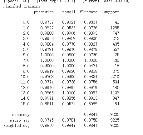
 　　HybridSN网络分类结果不同的原因是测试时不应使用dropout层和BN层。训练模式:model.train（）开启这两个层；测试模式:model.eval（）关闭这两个层。dropout层在训练过程中以指定概率p使神经元失活，让它在这次的传播过程的输出为0。当预测时要使用所有神经元而且要乘以一个补偿系数。所以要指定当前是训练还是测试模式。BN层在测试的时候采用的是固定的mean和var，这俩固定的参数是在训练时统计计算得到的。因为这俩参数是在前向传播过程中计算的，所以在测试模式的时候你如果没有指定model.eval（），那么这俩参数还会根据你的测试数据更新，导致结果的参考价值不大。综上，如果网络中添加了BN层和dropout层而不使用model.eval（）的话，每次测试的时候 模型并不是固定的，所以每次的分类结果并不一致。