Motivation 问题描述
对于一些问题标签值只有两个(1,0),而线性回归模型的输出值是一定范围的连续值。这时的做法是人为规定一个阈值0,当预测值大于0时判为1,预测值小于0时判为0.
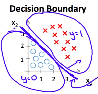 

上图对应的线性回归假设函数hypothesis为(特征的维数是2)
[h_ heta(x)=-3+x_1+x_2]
对于第i 个样例,当
[h_ heta(x^{(i)})>0]
预测为1,反之预测为0
使用这样的hypothesis带来的问题是无法定义损失函数。这时引入sigmoid函数。
[y = frac 1 {1+e^{-x}}]
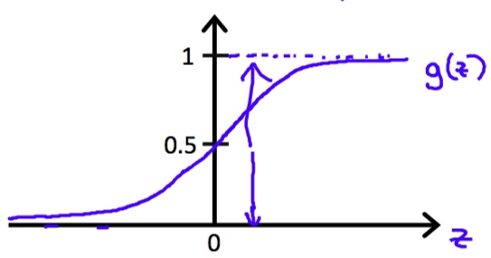 

Hypothesis
借助sigmoid函数,hypothesis定义为
[h_ heta(x) = frac 1 {1+e^{- heta x}}]
这时当
[ heta x > 0]
时,预测值归为1,此时有
[h_ heta(x)>0.5]
反之,当
[ heta x < 0]
时,预测值归为0,此时有
[h_ heta(x)<0.5]
Cost function
这样做的好处是
1. 使假设函数hypothesis的值落在区间(0,1)内。
2. 方便构造损失函数。
假设第i 个样本的标签为1的,当假设函数预测为0.7,他表示有70%的概率预测为1.使用极大似然估计这时此样本造成的损失为
[-1 imes{log0.7}]
而且当预测假设函数值为0.6时损失值
[-1 imes{log0.6}]
更大,这符合直观的认知。所以对于所有样本标签为1的样本,其损失函数定义为
[Cost(h_ heta(x^{(i)}),y^{(i)})=-y^{(i)}logh_ heta(x^{(i)})]
 

对于所有样本标签为0的样本,其损失函数定义为
[Cost(h_ heta(x^{(i)}),y^{(i)})=-(1-y^{(i)})log(1-h_ heta(x^{(i)}))]
 

可以看出当预测值为0时,其造成的损失为0;当预测值越大,其造成的损失也越大。综合以上两种情况,给出损失函数cost function的定义
[J( heta)=frac 1 msum_{i=1}^mCost(h_ heta(x^{(i)}),y^{(i)})
][=-frac 1 m[sum_{i=1}^my^{(i)}logh_ heta(x^{(i)})+(1-y^{(i)})log(1-h_ heta(x^{(i)}))]]
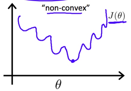
为什么不使用原来的平方差之和为损失函数?因为使用原来的损失函数可能会不收敛。

Gradient descent
碰巧的是梯度下降的公式和线性回归完全相同。代码实现的时候需要选择迭代次数和梯度下降速度参数alpha,这也是使用sigmoid函数的第三点好处。(此处省略证明)
[ heta_j := heta_j - alphafrac 1 {2m}sum_{i=1}^m(h_ heta(x^{(i)})-y^{(i)})cdot{x^{(i)}_j}]
实际情况是使用Matlab中的fminunc函数,它会自动选择参数alpha
Matlab 代码
Cost function with regularization
H = sigmoid(X*theta);
T = y.*log(H) + (1 - y).*log(1 - H);
J = -1/m*sum(T) + lambda/(2*m)*sum(theta(2:end).^2);
ta = [0; theta(2:end)];
grad = X'*(H - y)/m + lambda/m*ta;
Calculate parameters
[theta, cost] = fminunc(@(t)(costFunction(t, X, y)), initial_theta, options);
Predict
p = predict(theta, X);

fprintf('Train Accuracy: %f
', mean(double(p == y)) * 100);
function p = predict(theta, X)

m = size(X, 1); % Number of training examples
p = zeros(m, 1);

for i = 1:m
    temp = sigmoid(X(I,:)*theta);
    if temp>=0.5
        p(i,1)=1;
    else
        p(i,1)=0;
    end
end

end