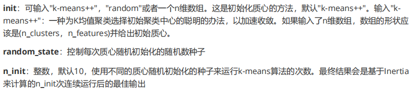
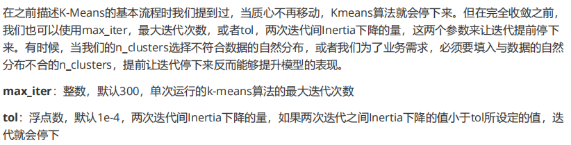
class sklearn.cluster.KMeans (n_clusters=8, init=’k-means++’, n_init=10, max_iter=300, tol=0.0001,precompute_distances=’auto’, verbose=0, random_state=None, copy_x=True, n_jobs=None, algorithm=’auto’)
1 重要参数n_clusters
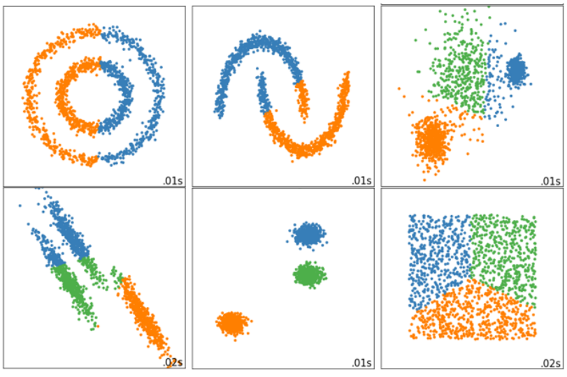
n_clusters是KMeans中的k,表示着我们告诉模型我们要分几类。这是KMeans当中唯一一个必填的参数,默认为8类,但通常我们的聚类结果会是一个小于8的结果。通常,在开始聚类之前,我们并不知道n_clusters究竟是多少,因此我们要对它进行探索。
1.1 先进行一次聚类看看吧
当我们拿到一个数据集,如果可能的话,我们希望能够通过绘图先观察一下这个数据集的数据分布,以此来为我们聚类时输入的n_clusters做一个参考。
首先,我们来自己创建一个数据集。这样的数据集是我们自己创建,所以是有标签的。
from sklearn.datasets import make_blobs
import matplotlib.pyplot as plt
#自己创建数据集
X, y = make_blobs(n_samples=500,n_features=2,centers=4,random_state=1)
fig, ax1 = plt.subplots(1)
ax1.scatter(X[:, 0], X[:, 1]
           ,marker='o' #点的形状
           ,s=8 #点的大小
           )
plt.show()
#如果我们想要看见这个点的分布,怎么办?
color = ["red","pink","orange","gray"]
fig, ax1 = plt.subplots(1)
for i in range(4):
    ax1.scatter(X[y==i, 0], X[y==i, 1]
           ,marker='o' #点的形状
           ,s=8 #点的大小
           ,c=color[i]
           )
plt.show()
基于这个分布,我们来使用Kmeans进行聚类。首先,我们要猜测一下,这个数据中有几簇?
from sklearn.cluster import KMeans
n_clusters = 3
cluster = KMeans(n_clusters=n_clusters, random_state=0).fit(X)
y_pred = cluster.labels_
y_pred
pre = cluster.fit_predict(X)
pre == y_pred

cluster_smallsub = KMeans(n_clusters=n_clusters, random_state=0).fit(X[:200])
y_pred_ = cluster_smallsub.predict(X)
y_pred == y_pred_

centroid = cluster.cluster_centers_
centroid

centroid.shape

inertia = cluster.inertia_
inertia

color = ["red","pink","orange","gray"]
fig, ax1 = plt.subplots(1)

for i in range(n_clusters):
    ax1.scatter(X[y_pred==i, 0], X[y_pred==i, 1]
           ,marker='o'
           ,s=8
           ,c=color[i]
           )
ax1.scatter(centroid[:,0],centroid[:,1]
           ,marker="x"
           ,s=15
           ,c="black")
plt.show()

n_clusters = 4
cluster_ = KMeans(n_clusters=n_clusters, random_state=0).fit(X)
inertia_ = cluster_.inertia_
inertia_

n_clusters = 5
cluster_ = KMeans(n_clusters=n_clusters, random_state=0).fit(X)
inertia_ = cluster_.inertia_
inertia_

n_clusters = 6
cluster_ = KMeans(n_clusters=n_clusters, random_state=0).fit(X)
inertia_ = cluster_.inertia_
inertia_
1.2 聚类算法的模型评估指标


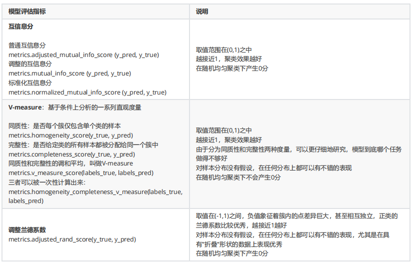
1.2.1 当真实标签已知的时候

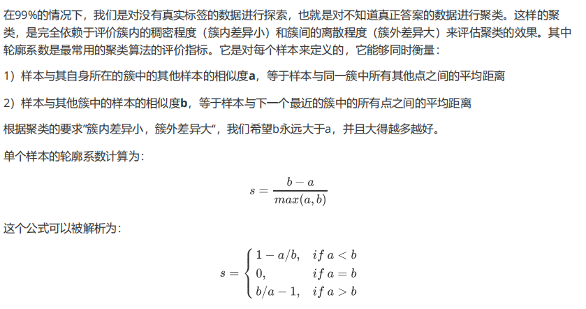
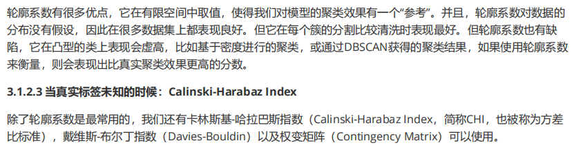
1.2.2 当真实标签未知的时候:轮廓系数


from sklearn.metrics import silhouette_score
from sklearn.metrics import silhouette_samples
X
y_pred
silhouette_score(X,y_pred)
silhouette_score(X,cluster_.labels_)
silhouette_samples(X,y_pred)

from sklearn.metrics import calinski_harabaz_score
X
y_pred
calinski_harabaz_score(X, y_pred)
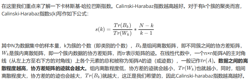
虽然calinski-Harabaz指数没有界,在凸型的数据上的聚类也会表现虚高。但是比起轮廓系数,它有一个巨大的优点,就是计算非常快速。之前我们使用过魔法命令%%timeit来计算一个命令的运算时间,今天我们来选择另一种方法:时间戳计算运行时间。
from time import time
t0 = time()
calinski_harabaz_score(X, y_pred)
time() - t0
t0 = time()
silhouette_score(X,y_pred)
time() - t0
import datetime
datetime.datetime.fromtimestamp(t0).strftime("%Y-%m-%d %H:%M:%S")
可以看得出,calinski-harabaz指数比轮廓系数的计算块了一倍不止。想想看我们使用的数据量,如果是一个以万计的数据,轮廓系数就会大大拖慢我们模型的运行速度了。
1.3 案例:基于轮廓系数来选择n_clusters
我们通常会绘制轮廓系数分布图和聚类后的数据分布图来选择我们的最佳n_clusters。
from sklearn.cluster import KMeans
from sklearn.metrics import silhouette_samples, silhouette_score
import matplotlib.pyplot as plt
import matplotlib.cm as cm
import numpy as np
n_clusters = 4
fig, (ax1, ax2) = plt.subplots(1, 2)
fig.set_size_inches(18, 7)
ax1.set_xlim([-0.1, 1])
ax1.set_ylim([0, X.shape[0] + (n_clusters + 1) * 10])
clusterer = KMeans(n_clusters=n_clusters, random_state=10).fit(X)
cluster_labels = clusterer.labels_
silhouette_avg = silhouette_score(X, cluster_labels)
print("For n_clusters =", n_clusters,
      "The average silhouette_score is :", silhouette_avg)
sample_silhouette_values = silhouette_samples(X, cluster_labels)
y_lower = 10
for i in range(n_clusters):
    ith_cluster_silhouette_values = sample_silhouette_values[cluster_labels == i]
    ith_cluster_silhouette_values.sort()
    size_cluster_i = ith_cluster_silhouette_values.shape[0]
    y_upper = y_lower + size_cluster_i
    color = cm.nipy_spectral(float(i)/n_clusters)
    ax1.fill_betweenx(np.arange(y_lower, y_upper)
                     ,ith_cluster_silhouette_values
                     ,facecolor=color
                     ,alpha=0.7
                     )
    ax1.text(-0.05
             , y_lower + 0.5 * size_cluster_i
             , str(i))
    y_lower = y_upper + 10
ax1.set_title("The silhouette plot for the various clusters.")
ax1.set_xlabel("The silhouette coefficient values")
ax1.set_ylabel("Cluster label")
ax1.axvline(x=silhouette_avg, color="red", linestyle="--")
ax1.set_yticks([])
ax1.set_xticks([-0.1, 0, 0.2, 0.4, 0.6, 0.8, 1])
colors = cm.nipy_spectral(cluster_labels.astype(float) / n_clusters)
ax2.scatter(X[:, 0], X[:, 1]
           ,marker='o'
           ,s=8
           ,c=colors
           )
centers = clusterer.cluster_centers_
# Draw white circles at cluster centers
ax2.scatter(centers[:, 0], centers[:, 1], marker='x',
            c="red", alpha=1, s=200)
ax2.set_title("The visualization of the clustered data.")
ax2.set_xlabel("Feature space for the 1st feature")
ax2.set_ylabel("Feature space for the 2nd feature")
plt.suptitle(("Silhouette analysis for KMeans clustering on sample data "
              "with n_clusters = %d" % n_clusters),
             fontsize=14, fontweight='bold')
plt.show()
将上述过程包装成一个循环,可以得到:
from sklearn.cluster import KMeans
from sklearn.metrics import silhouette_samples, silhouette_score
import matplotlib.pyplot as plt
import matplotlib.cm as cm
import numpy as np
for n_clusters in [2,3,4,5,6,7]:
    n_clusters = n_clusters
    fig, (ax1, ax2) = plt.subplots(1, 2)
    fig.set_size_inches(18, 7)
    ax1.set_xlim([-0.1, 1])
    ax1.set_ylim([0, X.shape[0] + (n_clusters + 1) * 10])
    clusterer = KMeans(n_clusters=n_clusters, random_state=10).fit(X)
    cluster_labels = clusterer.labels_
    silhouette_avg = silhouette_score(X, cluster_labels)
    print("For n_clusters =", n_clusters,
          "The average silhouette_score is :", silhouette_avg)
    sample_silhouette_values = silhouette_samples(X, cluster_labels)
    y_lower = 10
    for i in range(n_clusters):
        ith_cluster_silhouette_values = sample_silhouette_values[cluster_labels == i]
        ith_cluster_silhouette_values.sort()
        size_cluster_i = ith_cluster_silhouette_values.shape[0]
        y_upper = y_lower + size_cluster_i
        color = cm.nipy_spectral(float(i)/n_clusters)
        ax1.fill_betweenx(np.arange(y_lower, y_upper)
                         ,ith_cluster_silhouette_values
                         ,facecolor=color
                         ,alpha=0.7
                         )
        ax1.text(-0.05
                 , y_lower + 0.5 * size_cluster_i
                 , str(i))
        y_lower = y_upper + 10
    ax1.set_title("The silhouette plot for the various clusters.")
    ax1.set_xlabel("The silhouette coefficient values")
    ax1.set_ylabel("Cluster label")
    ax1.axvline(x=silhouette_avg, color="red", linestyle="--")
    ax1.set_yticks([])
    ax1.set_xticks([-0.1, 0, 0.2, 0.4, 0.6, 0.8, 1])
    colors = cm.nipy_spectral(cluster_labels.astype(float) / n_clusters)
    ax2.scatter(X[:, 0], X[:, 1]
               ,marker='o'
               ,s=8
               ,c=colors
               )
    centers = clusterer.cluster_centers_
    # Draw white circles at cluster centers
    ax2.scatter(centers[:, 0], centers[:, 1], marker='x',
                c="red", alpha=1, s=200)

    ax2.set_title("The visualization of the clustered data.")
    ax2.set_xlabel("Feature space for the 1st feature")
    ax2.set_ylabel("Feature space for the 2nd feature")
    plt.suptitle(("Silhouette analysis for KMeans clustering on sample data "
                  "with n_clusters = %d" % n_clusters),
                 fontsize=14, fontweight='bold')
    plt.show()
2 重要参数init & random_state & n_init:初始质心怎么放好?

X
y
plus = KMeans(n_clusters = 10).fit(X)
plus.n_iter_
random = KMeans(n_clusters = 10,init="random",random_state=420).fit(X)
random.n_iter_
3 重要参数max_iter & tol:让迭代停下来
random = KMeans(n_clusters = 10,init="random",max_iter=10,random_state=420).fit(X)
y_pred_max10 = random.labels_
silhouette_score(X,y_pred_max10)
random = KMeans(n_clusters = 10,init="random",max_iter=20,random_state=420).fit(X)
y_pred_max20 = random.labels_
silhouette_score(X,y_pred_max20)
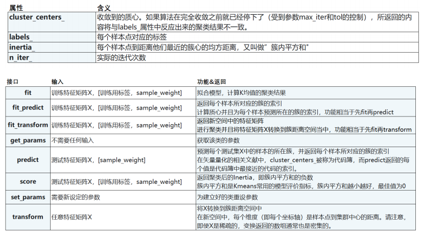
4 重要属性与重要接口

5 函数cluster.k_means
sklearn.cluster.k_means (X, n_clusters, sample_weight=None, init=’k-means++’, precompute_distances=’auto’,n_init=10, max_iter=300, verbose=False, tol=0.0001, random_state=None, copy_x=True, n_jobs=None,algorithm=’auto’, return_n_iter=False)
函数k_means的用法其实和类非常相似,不过函数是输入一系列值,而直接返回结果。一次性地,函数k_means会依次返回质心,每个样本对应的簇的标签,inertia以及最佳迭代次数。
from sklearn.cluster import k_means
k_means(X,4,return_n_iter=True)