YOLOv1是一个anchor-free的,从YOLOv2开始引入了Anchor,在VOC2007数据集上将mAP提升了10个百分点。YOLOv3也继续使用了Anchor,本文主要讲ultralytics版YOLOv3的Loss部分的计算, 实际上这部分loss和原版差距非常大,并且可以通过arc指定loss的构建方式, 如果想看原版的loss可以在下方release的v6中下载源码。
Github地址: https://github.com/ultralytics/yolov3
Github release: https://github.com/ultralytics/yolov3/releases
1. Anchor
Faster R-CNN中Anchor的大小和比例是由人手工设计的,可能并不贴合数据集,有可能会给模型性能带来负面影响。YOLOv2和YOLOv3则是通过聚类算法得到最适合的k个框。聚类距离是通过IoU来定义,IoU越大,边框距离越近。
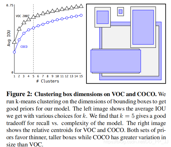
Anchor越多,平均IoU会越大,效果越好,但是会带来计算量上的负担,下图是YOLOv2论文中的聚类数量和平均IoU的关系图,在YOLOv2中选择了5个anchor作为精度和速度的平衡。
2. 偏移公式
在Faster RCNN中,中心坐标的偏移公式是:
其中(x_a)、(y_a) 代表中心坐标,(w_a)和(h_a)代表宽和高,(t_x)和(t_y)是模型预测的Anchor相对于Ground Truth的偏移量,通过计算得到的x,y就是最终预测框的中心坐标。
而在YOLOv2和YOLOv3中,对偏移量进行了限制,如果不限制偏移量,那么边框的中心可以在图像任何位置,可能导致训练的不稳定。
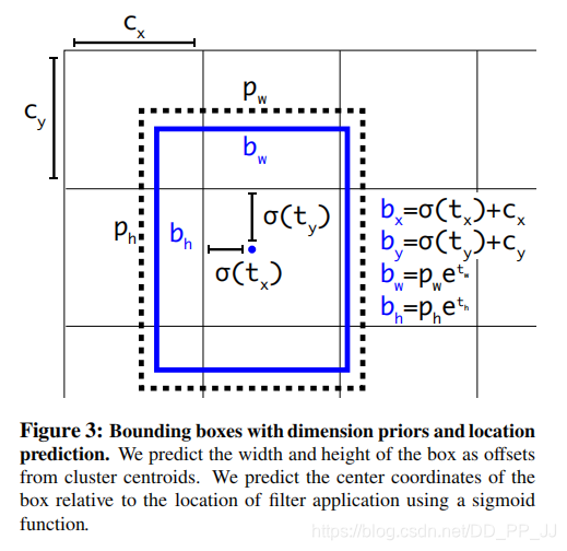
对照上图进行理解:
-
(c_x)和(c_y)分别代表中心点所处区域的左上角坐标。
-
(p_w)和(p_h)分别代表Anchor的宽和高。
-
(sigma(t_x))和(sigma(t_y))分别代表预测框中心点和左上角的距离,(sigma)代表sigmoid函数,将偏移量限制在当前grid中,有利于模型收敛。
-
(t_w)和(t_h)代表预测的宽高偏移量,Anchor的宽和高乘上指数化后的宽高,对Anchor的长宽进行调整。
-
(sigma(t_o))是置信度预测值,是当前框有目标的概率乘以bounding box和ground truth的IoU的结果
3. Loss
YOLOv3中有一个参数是ignore_thresh,在ultralytics版版的YOLOv3中对应的是train.py文件中的iou_t参数(默认为0.225)。
正负样本是按照以下规则决定的:
-
如果一个预测框与所有的Ground Truth的最大IoU<ignore_thresh时,那这个预测框就是负样本。
-
如果Ground Truth的中心点落在一个区域中,该区域就负责检测该物体。将与该物体有最大IoU的预测框作为正样本(注意这里没有用到ignore thresh,即使该最大IoU<ignore thresh也不会影响该预测框为正样本)
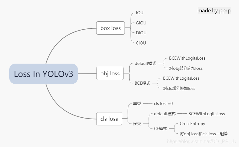
在YOLOv3中,Loss分为三个部分:
- 一个是xywh部分带来的误差,也就是bbox带来的loss
- 一个是置信度带来的误差,也就是obj带来的loss
- 最后一个是类别带来的误差,也就是class带来的loss
在代码中分别对应lbox, lobj, lcls,yolov3中使用的loss公式如下:
其中:
S: 代表grid size, (S^2)代表13x13,26x26, 52x52
B: box
(1_{i,j}^{obj}): 如果在i,j处的box有目标,其值为1,否则为0
(1_{i,j}^{noobj}): 如果在i,j处的box没有目标,其值为1,否则为0
BCE(binary cross entropy)具体计算公式如下:
以上是论文中yolov3对应的darknet。而pytorch版本的yolov3改动比较大,有较大的改动空间,可以通过参数进行调整。
分成三个部分进行具体分析:
1. lbox部分
在ultralytics版版的YOLOv3中,使用的是GIOU,具体讲解见GIOU讲解链接。
简单来说是这样的公式,IoU公式如下:
而GIoU公式如下:
其中(A_c)代表两个框最小闭包区域面积,也就是同时包含了预测框和真实框的最小框的面积。
yolov3中提供了IoU、GIoU、DIoU和CIoU等计算方式,以GIoU为例:
if GIoU:  # Generalized IoU https://arxiv.org/pdf/1902.09630.pdf
    c_area = cw * ch + 1e-16  # convex area
    return iou - (c_area - union) / c_area  # GIoU
可以看到代码和GIoU公式是一致的,再来看一下lbox计算部分:
giou = bbox_iou(pbox.t(), tbox[i],
				x1y1x2y2=False, GIoU=True)
lbox += (1.0 - giou).sum() if red == 'sum' else (1.0 - giou).mean()
可以看到box的loss是1-giou的值。
2. lobj部分
lobj代表置信度,即该bounding box中是否含有物体的概率。在yolov3代码中obj loss可以通过arc来指定,有两种模式:
如果采用default模式,使用BCEWithLogitsLoss,将obj loss和cls loss分开计算:
BCEobj = nn.BCEWithLogitsLoss(pos_weight=ft([h['obj_pw']]), reduction=red)
if 'default' in arc:  # separate obj and cls
    lobj += BCEobj(pi[..., 4], tobj)  # obj loss
    # pi[...,4]对应的是该框中含有目标的置信度,和giou计算BCE
    # 相当于将obj loss和cls loss分开计算
如果采用BCE模式,使用的也是BCEWithLogitsLoss, 计算对象是所有的cls loss:
BCE = nn.BCEWithLogitsLoss(reduction=red)
elif 'BCE' in arc:  # unified BCE (80 classes)
    t = torch.zeros_like(pi[..., 5:])  # targets
    if nb:
        t[b, a, gj, gi, tcls[i]] = 1.0 # 对应正样本class置信度设置为1
        lobj += BCE(pi[..., 5:], t)#pi[...,5:]对应的是所有的class
3. lcls部分
如果是单类的情况,cls loss=0
如果是多类的情况,也分两个模式:
如果采用default模式,使用的是BCEWithLogitsLoss计算class loss。
BCEcls = nn.BCEWithLogitsLoss(pos_weight=ft([h['cls_pw']]), reduction=red)
# cls loss 只计算多类之间的loss,单类不进行计算
if 'default' in arc and model.nc > 1:
    t = torch.zeros_like(ps[:, 5:])  # targets
    t[range(nb), tcls[i]] = 1.0 # 设置对应class为1
    lcls += BCEcls(ps[:, 5:], t)  # 使用BCE计算分类loss
如果采用CE模式,使用的是CrossEntropy同时计算obj loss和cls loss。
CE = nn.CrossEntropyLoss(reduction=red)
elif 'CE' in arc:  # unified CE (1 background + 80 classes)
    t = torch.zeros_like(pi[..., 0], dtype=torch.long)  # targets
    if nb:
    t[b, a, gj, gi] = tcls[i] + 1 # 由于cls是从零开始计数的,所以+1
    lcls += CE(pi[..., 4:].view(-1, model.nc + 1), t.view(-1))
    # 这里将obj loss和cls loss一起计算,使用CrossEntropy Loss
以上三部分总结下来就是下图:
4. 代码
ultralytics版版的yolov3的loss已经和论文中提出的部分大相径庭了,代码中很多地方地方是来自作者的经验。另外,这里读的代码是2020年2月份左右作者发布的版本,关注这个库的人会知道,作者更新速度非常快,在笔者写这篇文章的时候,loss也出现了大幅改动,添加了label smoothing等新的机制,去掉了通过arc来调整loss的机制,简化了loss部分。
这部分的代码添加了大量注释,很多是笔者通过debug得到的结果,理解的时候需要讲一下debug的配置:
- 单类数据集class=1
- batch size=2
- 模型是yolov3.cfg
计算loss这部分代码可以大概上分为两部分,一部分是正负样本选取,一部分是loss计算。
1. 正负样本选取部分
这部分主要工作是在每个yolo层将预设的anchor和ground truth进行匹配,得到正样本,回顾一下上文中在YOLOv3中正负样本选取规则:
-
如果一个预测框与所有的Ground Truth的最大IoU<ignore_thresh时,那这个预测框就是负样本。
-
如果Ground Truth的中心点落在一个区域中,该区域就负责检测该物体。将与该物体有最大IoU的预测框作为正样本(注意这里没有用到ignore thresh,即使该最大IoU<ignore thresh也不会影响该预测框为正样本)
def build_targets(model, targets):
    # targets = [image, class, x, y, w, h]
    # 这里的image是一个数字,代表是当前batch的第几个图片
    # x,y,w,h都进行了归一化,除以了宽或者高

    nt = len(targets)

    tcls, tbox, indices, av = [], [], [], []

    multi_gpu = type(model) in (nn.parallel.DataParallel,
                                nn.parallel.DistributedDataParallel)

    reject, use_all_anchors = True, True
    for i in model.yolo_layers:
        # yolov3.cfg中有三个yolo层,这部分用于获取对应yolo层的grid尺寸和anchor大小
        # ng 代表num of grid (13,13) anchor_vec [[x,y],[x,y]]
        # 注意这里的anchor_vec: 假如现在是yolo第一个层(downsample rate=32)
        # 这一层对应anchor为:[116, 90], [156, 198], [373, 326]
        # anchor_vec实际值为以上除以32的结果:[3.6,2.8],[4.875,6.18],[11.6,10.1]
        # 原图 416x416 对应的anchor为 [116, 90]
        # 下采样32倍后 13x13 对应的anchor为 [3.6,2.8]
        if multi_gpu:
            ng = model.module.module_list[i].ng
            anchor_vec = model.module.module_list[i].anchor_vec
        else:
            ng = model.module_list[i].ng,
            anchor_vec = model.module_list[i].anchor_vec

        # iou of targets-anchors
        # targets中保存的是ground truth
        t, a = targets, []

        gwh = t[:, 4:6] * ng[0]

        if nt:  # 如果存在目标
            # anchor_vec: shape = [3, 2] 代表3个anchor
            # gwh: shape = [2, 2] 代表 2个ground truth
            # iou: shape = [3, 2] 代表 3个anchor与对应的两个ground truth的iou
            iou = wh_iou(anchor_vec, gwh)  # 计算先验框和GT的iou

            if use_all_anchors:
                na = len(anchor_vec)  # number of anchors
                a = torch.arange(na).view(
                    (-1, 1)).repeat([1, nt]).view(-1)  # 构造 3x2 -> view到6
                # a = [0,0,1,1,2,2]
                t = targets.repeat([na, 1])
                # targets: [image, cls, x, y, w, h]
                # 复制3个: shape[2,6] to shape[6,6]
                gwh = gwh.repeat([na, 1])
                # gwh shape:[6,2]
            else:  # use best anchor only
                iou, a = iou.max(0)  # best iou and anchor
                # 取iou最大值是darknet的默认做法,返回的a是下角标

            # reject anchors below iou_thres (OPTIONAL, increases P, lowers R)
            if reject:
                # 在这里将所有阈值小于ignore thresh的去掉
                j = iou.view(-1) > model.hyp['iou_t']
                # iou threshold hyperparameter
                t, a, gwh = t[j], a[j], gwh[j]

        # Indices
        b, c = t[:, :2].long().t()  # target image, class
        # 取的是targets[image, class, x,y,w,h]中 [image, class]

        gxy = t[:, 2:4] * ng[0]  # grid x, y

        gi, gj = gxy.long().t()  # grid x, y indices
        # 注意这里通过long将其转化为整形,代表格子的左上角

        indices.append((b, a, gj, gi))
        # indice结构体保存内容为:
        '''
        b: 一个batch中的角标
        a: 代表所选中的正样本的anchor的下角标
        gj, gi: 代表所选中的grid的左上角坐标
        '''
        # Box
        gxy -= gxy.floor()  # xy
        # 现在gxy保存的是偏移量,是需要YOLO进行拟合的对象
        tbox.append(torch.cat((gxy, gwh), 1))  # xywh (grids)
        # 保存对应偏移量和宽高(对应13x13大小的)
        av.append(anchor_vec[a])  # anchor vec
        # av 是anchor vec的缩写,保存的是匹配上的anchor的列表

        # Class
        tcls.append(c)
        # tcls用于保存匹配上的类别列表
        if c.shape[0]:  # if any targets
            assert c.max() < model.nc, 'Model accepts %g classes labeled from 0-%g, however you labelled a class %g. '
                                       'See https://github.com/ultralytics/yolov3/wiki/Train-Custom-Data' % (
                                           model.nc, model.nc - 1, c.max())
    return tcls, tbox, indices, av
梳理一下在每个YOLO层的匹配流程:
- 将ground truth和anchor进行匹配,得到iou
- 然后有两个方法匹配:
- 使用yolov3原版的匹配机制,仅仅选择iou最大的作为正样本
- 使用ultralytics版版yolov3的默认匹配机制,use_all_anchors=True的时候,选择所有的匹配对
- 对以上匹配的部分在进行筛选,对应原版yolo中ignore_thresh部分,将以上匹配到的部分中iou<ignore_thresh的部分筛选掉。
- 最后将匹配得到的内容返回到compute_loss函数中。
2. loss计算部分
这部分就是yolov3中核心loss计算,这部分对照上文的讲解进行理解。
def compute_loss(p, targets, model):
    # p: (bs, anchors, grid, grid, classes + xywh)
    # predictions, targets, model
    ft = torch.cuda.FloatTensor if p[0].is_cuda else torch.Tensor
    lcls, lbox, lobj = ft([0]), ft([0]), ft([0])
    tcls, tbox, indices, anchor_vec = build_targets(model, targets)
    '''
    以yolov3为例,有三个yolo层
    tcls: 一个list保存三个tensor,每个tensor中有6(2个gtx3个anchor)个代表类别的数字
    tbox: 一个list保存三个tensor,每个tensor形状[6,4],6(2个gtx3个anchor)个bbox
    indices: 一个list保存三个tuple,每个tuple中保存4个tensor:
            分别代表        b: 一个batch中的角标
                            a: 代表所选中的正样本的anchor的下角标
                            gj, gi: 代表所选中的grid的左上角坐标
    anchor_vec: 一个list保存三个tensor,每个tensor形状[6,2],
                6(2个gtx3个anchor)个anchor,注意大小是相对于13x13feature map的anchor大小
    '''

    h = model.hyp  # hyperparameters
    arc = model.arc  # # (default, uCE, uBCE) detection architectures
    # 具体使用的损失函数是通过arc参数决定的
    red = 'sum'  # Loss reduction (sum or mean)

    # Define criteria
    BCEcls = nn.BCEWithLogitsLoss(pos_weight=ft([h['cls_pw']]), reduction=red)
    BCEobj = nn.BCEWithLogitsLoss(pos_weight=ft([h['obj_pw']]), reduction=red)
    #BCEWithLogitsLoss = sigmoid + BCELoss
    BCE = nn.BCEWithLogitsLoss(reduction=red)
    CE = nn.CrossEntropyLoss(reduction=red)  # weight=model.class_weights

    # class label smoothing https://arxiv.org/pdf/1902.04103.pdf eqn 3
    # cp, cn = smooth_BCE(eps=0.0)
    # 这是最新的版本中提供了label smoothing的功能,只能用在多类问题

    if 'F' in arc:  # add focal loss
        g = h['fl_gamma']
        BCEcls, BCEobj, BCE, CE = FocalLoss(BCEcls, g), FocalLoss(
            BCEobj, g), FocalLoss(BCE, g), FocalLoss(CE, g)
        # focal loss可以用在cls loss或者obj loss

    # Compute losses
    np, ng = 0, 0  # number grid points, targets
    # np这个命名真的迷,建议改一下和numpy缩写重复
    for i, pi in enumerate(p):  # layer index, layer predictions
        # 在yolov3中,p有三个yolo layer的输出pi
        # 形状为:(bs, anchors, grid, grid, classes + xywh)
        b, a, gj, gi = indices[i]  # image, anchor, gridy, gridx
        tobj = torch.zeros_like(pi[..., 0])
        # tobj = target obj, 形状为(bs, anchors, grid, grid)
        np += tobj.numel() # 返回tobj中元素个数

        # Compute losses
        nb = len(b)
        if nb:
            ng += nb # number of targets 用于最后算平均loss
            # (bs, anchors, grid, grid, classes + xywh)
            ps = pi[b, a, gj, gi] # 即找到了对应目标的classes+xywh,形状为[6(2x3),6]

            # GIoU
            pxy = torch.sigmoid(
                ps[:, 0:2] # 将x,y进行sigmoid
            )  # pxy = pxy * s - (s - 1) / 2,  s = 1.5  (scale_xy)
            pwh = torch.exp(ps[:, 2:4]).clamp(max=1E3) * anchor_vec[i]
            # 防止溢出进行clamp操作,乘以13x13feature map对应的anchor
            # 这部分和上文中偏移公式是一致的
            pbox = torch.cat((pxy, pwh), 1)  # predicted box
            # pbox: predicted bbox shape:[6, 4]
            giou = bbox_iou(pbox.t(), tbox[i], x1y1x2y2=False,
                            GIoU=True)  # giou computation
            # 计算giou loss, 形状为6
            lbox += (1.0 - giou).sum() if red == 'sum' else (1.0 - giou).mean()
            # bbox loss直接由giou决定
            tobj[b, a, gj, gi] = giou.detach().type(tobj.dtype)
            # target obj 用giou取代1,代表该点对应置信度

            # cls loss 只计算多类之间的loss,单类不进行计算
            if 'default' in arc and model.nc > 1:
                t = torch.zeros_like(ps[:, 5:])  # targets
                t[range(nb), tcls[i]] = 1.0 # 设置对应class为1
                lcls += BCEcls(ps[:, 5:], t)  # 使用BCE计算分类loss

        if 'default' in arc:  # separate obj and cls
            lobj += BCEobj(pi[..., 4], tobj)  # obj loss
            # pi[...,4]对应的是该框中含有目标的置信度,和giou计算BCE
            # 相当于将obj loss和cls loss分开计算

        elif 'BCE' in arc:  # unified BCE (80 classes)
            t = torch.zeros_like(pi[..., 5:])  # targets
            if nb:
                t[b, a, gj, gi, tcls[i]] = 1.0 # 对应正样本class置信度设置为1
            lobj += BCE(pi[..., 5:], t)
            #pi[...,5:]对应的是所有的class

        elif 'CE' in arc:  # unified CE (1 background + 80 classes)
            t = torch.zeros_like(pi[..., 0], dtype=torch.long)  # targets
            if nb:
                t[b, a, gj, gi] = tcls[i] + 1 # 由于cls是从零开始计数的,所以+1
            lcls += CE(pi[..., 4:].view(-1, model.nc + 1), t.view(-1))
            # 这里将obj loss和cls loss一起计算,使用CrossEntropy Loss
    # 使用对应的权重来平衡,这个参数是作者通过参数搜索(random search)的方法搜索得到的
    lbox *= h['giou']
    lobj *= h['obj']
    lcls *= h['cls']

    if red == 'sum':
        bs = tobj.shape[0]  # batch size
        lobj *= 3 / (6300 * bs) * 2
        # 6300 = (10 ** 2 + 20 ** 2 + 40 ** 2) * 3
        # 输入为320x320的图片,则存在6300个anchor
        # 3代表3个yolo层, 2是一个超参数,通过实验获取
        # 如果不想计算的话,可以修改red='mean'
        if ng:
            lcls *= 3 / ng / model.nc
            lbox *= 3 / ng
    loss = lbox + lobj + lcls
    return loss, torch.cat((lbox, lobj, lcls, loss)).detach()
需要注意的是,三个部分的loss的平衡权重不是按照yolov3原文的设置来做的,是通过超参数进化来搜索得到的,具体请看:【从零开始学习YOLOv3】4. YOLOv3中的参数进化
5. 补充
补充一下BCEWithLogitsLoss的用法,在这之前先看一下BCELoss:
torch.nn.BCELoss的功能是二分类任务是的交叉熵计算函数,可以认为是CrossEntropy的特例。其分类限定为二分类,y的值必须为{0,1},input应该是概率分布的形式。在使用BCELoss前一般会先加一个sigmoid激活层,常用在自编码器中。
计算公式:
(w_n)是每个类别的loss权重,用于类别不均衡问题。
torch.nn.BCEWithLogitsLoss的相当于Sigmoid+BCELoss, 即input会经过Sigmoid激活函数,将input变为概率分布的形式。
计算公式: