PyTorch实现简单的自动编码器autoencoder

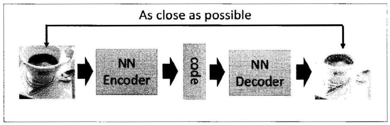
      自动编码器包括编码器(Encoder)和解码器(Decoder)两部分，编码器和解码器都可以是任意的模型，目前神经网络模型用的较多。输入的数据经过神经网络降维到一个编码(coder)，然后又通过一个神经网络去解码得到一个与原输入数据一模一样的生成数据，然后通过比较这两个数据，最小化它们之间的差异来训练这个网络中的编码器和解码器的参数，当这个过程训练完之后，拿出这个解码器，随机传入一个编码，通过解码器能够生成一个和原数据差不多的数据。^[1]

      莫烦的PyTorch系列教程^[2]中有关于自动编码器的介绍以及实现简单的自动编码器的代码。为方便查看，代码摘录如下：

import torch
import torch.nn as nn
import torch.utils.data as Data
import torchvision
import matplotlib.pyplot as plt
from mpl_toolkits.mplot3d import Axes3D
from matplotlib import cm
import numpy as np


# torch.manual_seed(1)    # reproducible

# Hyper Parameters
EPOCH = 10
BATCH_SIZE = 64
LR = 0.005         # learning rate
DOWNLOAD_MNIST = False
N_TEST_IMG = 5

# Mnist digits dataset
train_data = torchvision.datasets.MNIST(
    root='/Users/wangpeng/Desktop/all/CS/Courses/Deep Learning/mofan_PyTorch/mnist/',    # mnist has been downloaded before, use it directly
    train=True,                                     # this is training data
    transform=torchvision.transforms.ToTensor(),    # Converts a PIL.Image or numpy.ndarray to
                                                    # torch.FloatTensor of shape (C x H x W) and normalize in the range [0.0, 1.0]
    download=DOWNLOAD_MNIST,                        # download it if you don't have it
)

# plot one example
print(train_data.data.size())     # (60000, 28, 28)
print(train_data.targets.size())   # (60000)
plt.imshow(train_data.data[2].numpy(), cmap='gray')
plt.title('%i' % train_data.targets[2])
plt.show()

# Data Loader for easy mini-batch return in training, the image batch shape will be (50, 1, 28, 28)
train_loader = Data.DataLoader(dataset=train_data, batch_size=BATCH_SIZE, shuffle=True)


class AutoEncoder(nn.Module):
    def __init__(self):
        super(AutoEncoder, self).__init__()

        self.encoder = nn.Sequential(
            nn.Linear(28*28, 128),
            nn.Tanh(),
            nn.Linear(128, 64),
            nn.Tanh(),
            nn.Linear(64, 12),
            nn.Tanh(),
            nn.Linear(12, 3),   # compress to 3 features which can be visualized in plt
        )
        self.decoder = nn.Sequential(
            nn.Linear(3, 12),
            nn.Tanh(),
            nn.Linear(12, 64),
            nn.Tanh(),
            nn.Linear(64, 128),
            nn.Tanh(),
            nn.Linear(128, 28*28),
            nn.Sigmoid(),       # compress to a range (0, 1)
        )

    def forward(self, x):
        encoded = self.encoder(x)
        decoded = self.decoder(encoded)
        return encoded, decoded


autoencoder = AutoEncoder()

optimizer = torch.optim.Adam(autoencoder.parameters(), lr=LR)
loss_func = nn.MSELoss()

# initialize figure
f, a = plt.subplots(2, N_TEST_IMG, figsize=(5, 2))    # f是一块画布；a是一个大小为2*5的数组，数组中的每个元素都是一个画图对象
plt.ion()   # Turn the interactive mode on, continuously plot

# original data (first row) for viewing
view_data = train_data.data[:N_TEST_IMG].view(-1, 28*28).type(torch.FloatTensor)/255.
for i in range(N_TEST_IMG):
    a[0][i].imshow(np.reshape(view_data.data.numpy()[i], (28, 28)), cmap='gray')
    a[0][i].set_xticks(()); a[0][i].set_yticks(())

for epoch in range(EPOCH):
    for step, (x, b_label) in enumerate(train_loader):
        b_x = x.view(-1, 28*28)   # batch x, shape (batch, 28*28)
        b_y = x.view(-1, 28*28)   # batch y, shape (batch, 28*28)

        encoded, decoded = autoencoder(b_x)

        loss = loss_func(decoded, b_y)      # mean square error
        optimizer.zero_grad()               # clear gradients for this training step
        loss.backward()                     # backpropagation, compute gradients
        optimizer.step()                    # apply gradients

        if step % 100 == 0:
            print('Epoch: ', epoch, '| train loss: %.4f' % loss.data.numpy())

            # plotting decoded image (second row)
            _, decoded_data = autoencoder(view_data)
            for i in range(N_TEST_IMG):
                a[1][i].clear()
                a[1][i].imshow(np.reshape(decoded_data.data.numpy()[i], (28, 28)), cmap='gray')
                a[1][i].set_xticks(())
                a[1][i].set_yticks(())
            plt.draw()
            plt.pause(0.02)

plt.ioff()   # Turn the interactive mode off
plt.show()

# visualize in 3D plot
view_data = train_data.data[:200].view(-1, 28*28).type(torch.FloatTensor)/255.
encoded_data, _ = autoencoder(view_data)
fig = plt.figure(2)
ax = Axes3D(fig)    # 3D 图
# x, y, z 的数据值
X = encoded_data.data[:, 0].numpy()
Y = encoded_data.data[:, 1].numpy()
Z = encoded_data.data[:, 2].numpy()
values = train_data.targets[:200].numpy()    # 标签值
for x, y, z, s in zip(X, Y, Z, values):
    c = cm.rainbow(int(255*s/9))    # 上色
    ax.text(x, y, z, s, backgroundcolor=c)    # 标位子
ax.set_xlim(X.min(), X.max())
ax.set_ylim(Y.min(), Y.max())
ax.set_zlim(Z.min(), Z.max())
plt.show()


# test the decoder with a random code
code = torch.FloatTensor([[1.7, -2.5, 3.1]])   # 随机给一个张量
decode = autoencoder.decoder(code)  # decode shape (1, 178)
decode = decode.view(decode.size()[0], 28, 28)
decode_img = decode.squeeze().data.numpy() * 255
plt.figure()
plt.imshow(decode_img.astype(np.uint8), cmap='gray')

 

参考资料：

[1] 深度学习之PyTorch，廖星宇

[2] 莫烦的PyTorch系列教程