使用TensorFlow v2.0构建卷积神经网络。
这个例子使用低级方法来更好地理解构建卷积神经网络和训练过程背后的所有机制。
CNN 概述

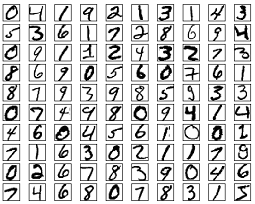
MNIST 数据集概述
此示例使用手写数字的MNIST数据集。该数据集包含60,000个用于训练的示例和10,000个用于测试的示例。这些数字已经过尺寸标准化并位于图像中心,图像是固定大小(28x28像素),值为0到255。
在此示例中,每个图像将转换为float32并归一化为[0,1]。
更多信息请查看链接: http://yann.lecun.com/exdb/mnist/
from __future__ import absolute_import, division, print_function

import tensorflow as tf
import numpy as np
# MNIST 数据集参数
num_classes = 10 # 所有类别(数字 0-9)

# 训练参数
learning_rate = 0.001
training_steps = 200
batch_size = 128
display_step = 10

# 网络参数
conv1_filters = 32 # 第一层卷积层卷积核的数目
conv2_filters = 64 # 第二层卷积层卷积核的数目
fc1_units = 1024 # 第一层全连接层神经元的数目
# 准备MNIST数据
from tensorflow.keras.datasets import mnist
(x_train, y_train), (x_test, y_test) = mnist.load_data()
# 转化为float32
x_train, x_test = np.array(x_train, np.float32), np.array(x_test, np.float32)
# 将图像值从[0,255]归一化到[0,1]
x_train, x_test = x_train / 255., x_test / 255.
# 使用tf.data API对数据进行随机排序和批处理
train_data = tf.data.Dataset.from_tensor_slices((x_train, y_train))
train_data = train_data.repeat().shuffle(5000).batch(batch_size).prefetch(1)
# 为简单起见创建一些包装器
def conv2d(x, W, b, strides=1):
    # Conv2D包装器, 带有偏置和relu激活
    x = tf.nn.conv2d(x, W, strides=[1, strides, strides, 1], padding='SAME')
    x = tf.nn.bias_add(x, b)
    return tf.nn.relu(x)

def maxpool2d(x, k=2):
    # MaxPool2D包装器
    return tf.nn.max_pool(x, ksize=[1, k, k, 1], strides=[1, k, k, 1], padding='SAME')
# 存储层的权重和偏置

# 随机值生成器初始化权重
random_normal = tf.initializers.RandomNormal()

weights = {
    # 第一层卷积层: 5 * 5卷积,1个输入, 32个卷积核(MNIST只有一个颜色通道)
    'wc1': tf.Variable(random_normal([5, 5, 1, conv1_filters])),
    # 第二层卷积层: 5 * 5卷积,32个输入, 64个卷积核
    'wc2': tf.Variable(random_normal([5, 5, conv1_filters, conv2_filters])),
    # 全连接层: 7*7*64 个输入, 1024个神经元
    'wd1': tf.Variable(random_normal([7*7*64, fc1_units])),
    # 全连接层输出层: 1024个输入, 10个神经元(所有类别数目)
    'out': tf.Variable(random_normal([fc1_units, num_classes]))
}

biases = {
    'bc1': tf.Variable(tf.zeros([conv1_filters])),
    'bc2': tf.Variable(tf.zeros([conv2_filters])),
    'bd1': tf.Variable(tf.zeros([fc1_units])),
    'out': tf.Variable(tf.zeros([num_classes]))
}
# 创建模型
def conv_net(x):

    # 输入形状:[-1, 28, 28, 1]。一批28*28*1(灰度)图像
    x = tf.reshape(x, [-1, 28, 28, 1])

    # 卷积层, 输出形状:[ -1, 28, 28 ,32]
    conv1 = conv2d(x, weights['wc1'], biases['bc1'])

    # 最大池化层(下采样) 输出形状:[ -1, 14, 14, 32]
    conv1 = maxpool2d(conv1, k=2)

    # 卷积层, 输出形状:[ -1, 14, 14, 64]
    conv2 = conv2d(conv1, weights['wc2'], biases['bc2'])

    # 最大池化层(下采样) 输出形状:[ -1, 7, 7, 64]
    conv2 = maxpool2d(conv2, k=2)

    # 修改conv2的输出以适应完全连接层的输入, 输出形状:[-1, 7*7*64]
    fc1 = tf.reshape(conv2, [-1, weights['wd1'].get_shape().as_list()[0]])

    # 全连接层, 输出形状: [-1, 1024]
    fc1 = tf.add(tf.matmul(fc1, weights['wd1']), biases['bd1'])
     # 将ReLU应用于fc1输出以获得非线性
    fc1 = tf.nn.relu(fc1)

    # 全连接层,输出形状 [ -1, 10]
    out = tf.add(tf.matmul(fc1, weights['out']), biases['out'])
    # 应用softmax将输出标准化为概率分布
    return tf.nn.softmax(out)
# 交叉熵损失函数
def cross_entropy(y_pred, y_true):
    # 将标签编码为独热向量
    y_true = tf.one_hot(y_true, depth=num_classes)
    # 将预测值限制在一个范围之内以避免log(0)错误
    y_pred = tf.clip_by_value(y_pred, 1e-9, 1.)
    # 计算交叉熵
    return tf.reduce_mean(-tf.reduce_sum(y_true * tf.math.log(y_pred)))

#  准确率评估
def accuracy(y_pred, y_true):
    # 预测类是预测向量中最高分的索引(即argmax)
    correct_prediction = tf.equal(tf.argmax(y_pred, 1), tf.cast(y_true, tf.int64))
    return tf.reduce_mean(tf.cast(correct_prediction, tf.float32), axis=-1)

# ADAM 优化器
optimizer = tf.optimizers.Adam(learning_rate)
# 优化过程
def run_optimization(x, y):
    # 将计算封装在GradientTape中以实现自动微分
    with tf.GradientTape() as g:
        pred = conv_net(x)
        loss = cross_entropy(pred, y)

    # 要更新的变量,即可训练的变量
    trainable_variables = weights.values()   biases.values()

    # 计算梯度
    gradients = g.gradient(loss, trainable_variables)

    # 按gradients更新 W 和 b
    optimizer.apply_gradients(zip(gradients, trainable_variables))
# 针对给定步骤数进行训练
for step, (batch_x, batch_y) in enumerate(train_data.take(training_steps), 1):
    # 运行优化以更新W和b值
    run_optimization(batch_x, batch_y)

    if step % display_step == 0:
        pred = conv_net(batch_x)
        loss = cross_entropy(pred, batch_y)
        acc = accuracy(pred, batch_y)
        print("step: %i, loss: %f, accuracy: %f" % (step, loss, acc))
output:
step: 10, loss: 72.370056, accuracy: 0.851562
step: 20, loss: 53.936745, accuracy: 0.882812
step: 30, loss: 29.929554, accuracy: 0.921875
step: 40, loss: 28.075102, accuracy: 0.953125
step: 50, loss: 19.366310, accuracy: 0.960938
step: 60, loss: 20.398090, accuracy: 0.945312
step: 70, loss: 29.320951, accuracy: 0.960938
step: 80, loss: 9.121045, accuracy: 0.984375
step: 90, loss: 11.680668, accuracy: 0.976562
step: 100, loss: 12.413654, accuracy: 0.976562
step: 110, loss: 6.675493, accuracy: 0.984375
step: 120, loss: 8.730624, accuracy: 0.984375
step: 130, loss: 13.608270, accuracy: 0.960938
step: 140, loss: 12.859011, accuracy: 0.968750
step: 150, loss: 9.110849, accuracy: 0.976562
step: 160, loss: 5.832032, accuracy: 0.984375
step: 170, loss: 6.996647, accuracy: 0.968750
step: 180, loss: 5.325038, accuracy: 0.992188
step: 190, loss: 8.866342, accuracy: 0.984375
step: 200, loss: 2.626245, accuracy: 1.000000
# 在验证集上测试模型
pred = conv_net(x_test)
print("Test Accuracy: %f" % accuracy(pred, y_test))
output:
Test Accuracy: 0.980000
# 可视化预测
import matplotlib.pyplot as plt
# 从验证集中预测5张图像
n_images = 5
test_images = x_test[:n_images]
predictions = conv_net(test_images)

# 显示图片和模型预测结果
for i in range(n_images):
    plt.imshow(np.reshape(test_images[i], [28, 28]), cmap='gray')
    plt.show()
    print("Model prediction: %i" % np.argmax(predictions.numpy()[i]))
output:
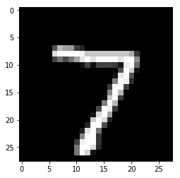
Model prediction: 7
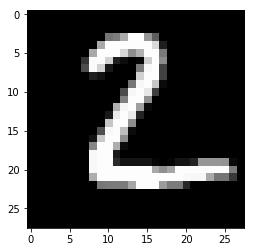
Model prediction:2
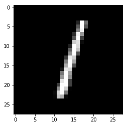
Model prediction: 1
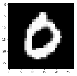
Model prediction: 0
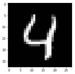
Model prediction: 4
欢迎关注磐创博客资源汇总站:
http://docs.panchuang.net/
欢迎关注PyTorch官方中文教程站:
http://pytorch.panchuang.net/