检测车道线——5.霍夫变换 Hough Transform

检测车道线——5.霍夫变换 Hough Transform
1、霍夫变换原理　

　　霍夫变换：从图像空间到霍夫空间的转换。

　　目的：是为了用参数空间表示图像空间中的线（图1）。

　　图1

　　在霍夫空间中，我可以将图像空间的“x vs. y”线表示为霍夫空间的“m vs. b”中的一个点。

　　因此，图像空间中一条线的表征将是霍夫空间中位置 (m, b) 处的单个点（图2）。

   图2

题1：

　　空间坐标系下，y=mx+b

变换到霍夫空间后，是图3哪种情况？

   图3

答案：C

理由：

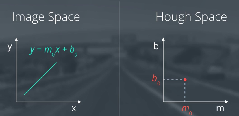
1、空间坐标系的直线转换到霍夫空间是点，因为直线的参数确定，确定的参数在霍夫空间里面就是点；m相同，b不同

2、b= -xm+y，两个及以上的（x，y）可以确定一个（m，b），所以笛卡尔坐标系里面的2条直线可以对应到霍夫空间里面的2个点。

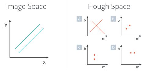
题2：

　　下图中，图像空间中的点对应于霍夫空间中的什么？

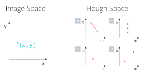
   图4

答案：A

解释：

1、空间坐标系的点转换到霍夫空间是直线，因为经过这个点有无穷个直线，每个直线对应的（m，b）不同，都经过同一个点。

2、b= -x₀m+y₀，是一条确定的直线。

题3：

　　下图中，图像空间中两点在霍夫空间中的表示是什么？

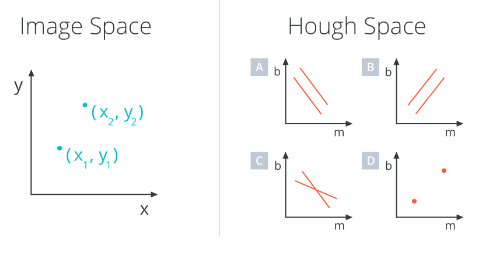
   图5

答案：C

解释：

1、图像空间中，任意2点都能经过一条直线，所以霍夫空间里面2条直线必有一个交点，即为共线的直线的参数；

2、b= -x₁m+y₁，b= -x₂m+y₂， 0> -x₁> -x₂， y₁< y₂

题4：

　　下图中，霍夫空间中两条线的交点在图像空间中对应什么？

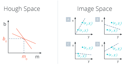
   图6

答案：A

解释：

1、霍夫空间中，两条直线代表图像空间的两个点，两条直线都经过（m₀，b₀），说明图像空间的两个点在参数为（m₀，b₀）的直线上；

2、m₀> 0，b₀ > 0，说明斜率为正、截距为正。

　　通过题3和题4可以看出，在图像空间中寻找线，可以通过在霍夫空间中寻找相交的线。

　　我们通过将霍夫空间划分为一个网格来做到这一点，并将相交线定义为通过给定网格单元的所有线。

　　首先运行 Canny 边缘检测算法来查找与图像中的边缘相关的所有点。

　　然后，我可以将这个边缘检测图像中的每个点视为霍夫空间中的一条线，如图7所示。在霍夫空间中的许多线相交的地方，可以说明找到了一组点（类比题3和题4），这些点描述了图像空间中的一条线。

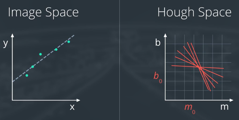
   图7

　　由于垂直线的斜率是无限大的，不利于计算，因此我们需要一个新的参数表达——通过极坐标重新定义直线，如图8所示。

　　ρ表示直线到原点的垂直距离，θ表示直线的垂线与横轴的夹角。

　　可以得到 x₀=ρ₀*cosθ₀y₀=ρ₀*sinθ₀ →   x₀*cosθ₀+y₀*sinθ₀ = ρ₀

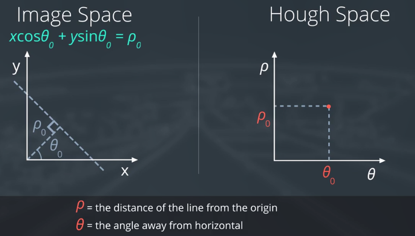
   图8

因为 x₀*cosθ+y₀*sinθ = ρ

　　现在图像空间中的每个点对应于霍夫空间中的一条正弦曲线。

假设x₀和y₀是（1,1）的情况下，x₀*cosθ+y₀*sinθ = ρ 如下图所示，可以看出是三角函数。

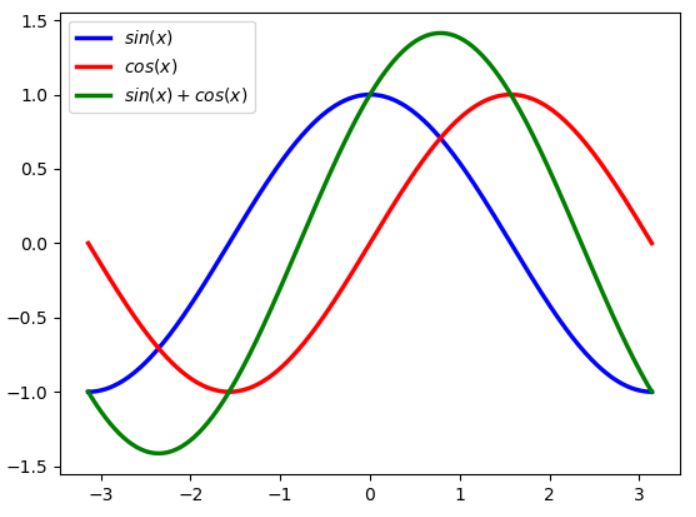
　　如果我们取一整条点，它会转化为霍夫空间中的一大堆正弦曲线。类比直线的情况，这些正弦曲线在霍夫空间中的交点，为图像空间直线的参数。
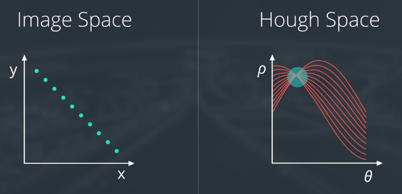
   图9

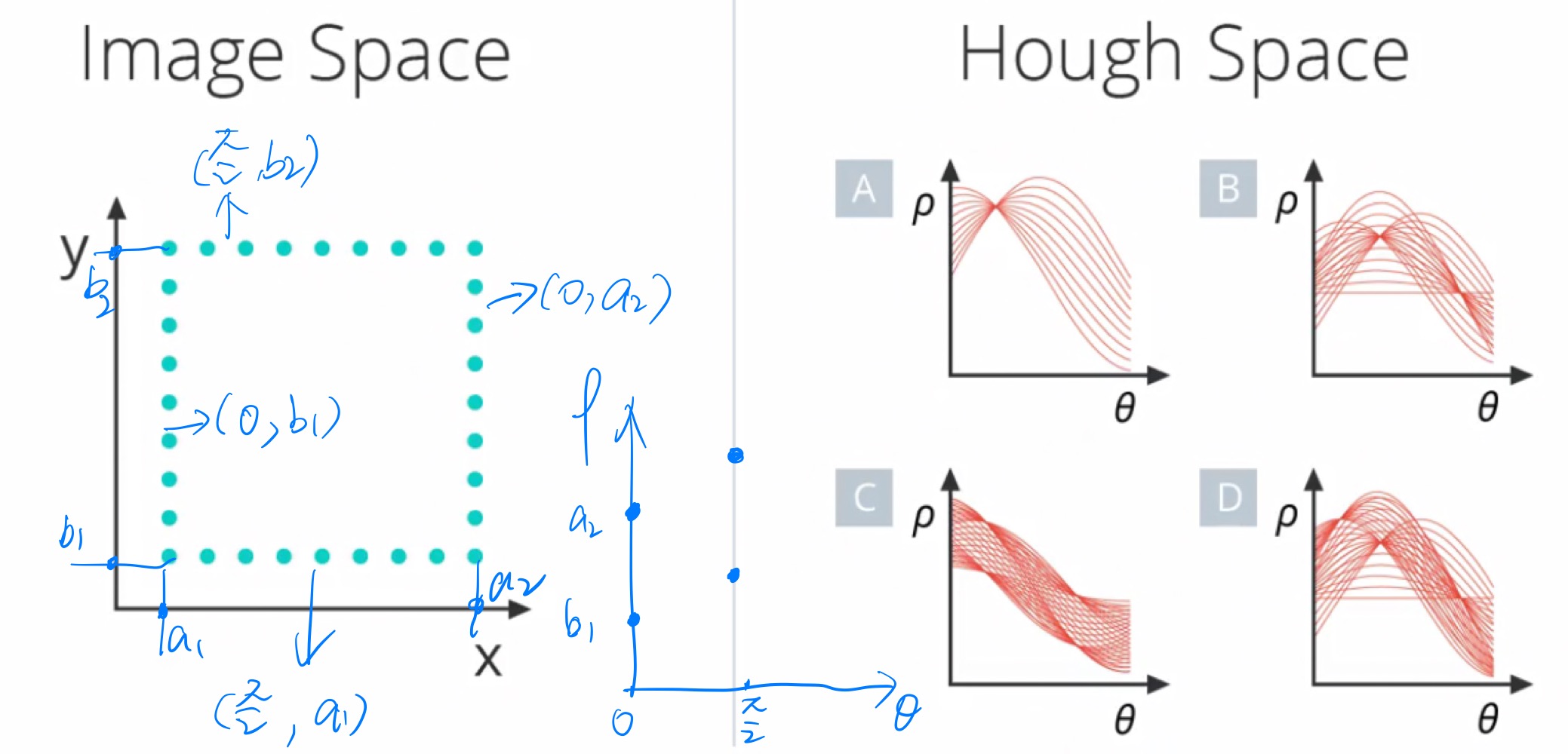
题5：

　　如果我们在正方形图像上运行霍夫变换会发生什么？霍夫空间中的对应图会是什么样子？

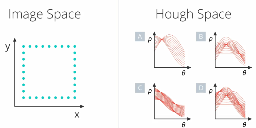
   图10

答案：C

解释：

1、图像空间有4条直线，说明霍夫空间有4个交点；

2、4个点（θ，ρ）为（0，ρ₁）、（0，ρ₂）、（π/2，ρ₁）、（π/2，ρ₂），可以看出，四个点。

  x₀*cosθ₀+y₀*sinθ₀ = ρ₀→ y = ρ₀- (cosθ₀/ sinθ₀) * x

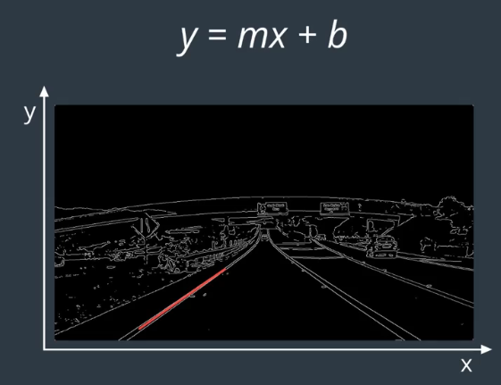
2、霍夫变换在车道线检测中的应用

　　车道线检测涉及更详细的车道线属性，例如长线、短线、弯曲线、虚线等。

　　在使用Canny function提取边缘的图像中，使用OpenCV的函数HoughLinesP( )。（相关资料可以参考OpenCV_Hough Line Transform和不用OpenCV求解Hough Transform的方法。）

HoughLinesP如下：
lines = cv2.HoughLinesP(edges, rho, theta, threshold, np.array([]), min_line_length, max_line_gap)
-- 附录--

1、进一步理解霍夫变换

　　笛卡尔坐标系下的直线如下所示。

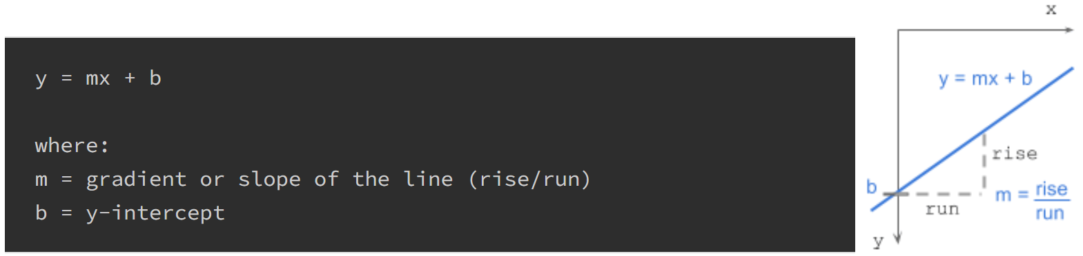
　　在笛卡尔图像空间中共线的点将在m-b(gradient-intercept)参数空间中相交。若图像空间所有点都在同一条直线上，表示相交在参数空间中的同一个点处。参数空间中的公共点 (m, b) 表示图像空间中的线。如下图所示，图像空间中某一点（x₁,y₁）处可能存在的所有的直线（蓝色）的(m,b)，对应到参数空间中蓝色直线 b= -mx₁+y₁ 中的（m,b）的值。

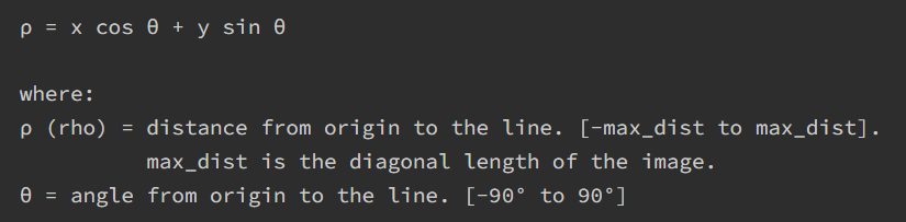
　　gradient-intercept参数空间中的斜率会无限大，所以转换到angle-distance参数空间——极坐标系。将笛卡尔坐标系中的 $y = m x + b$ 转为极坐标系的参数 $(ρ, θ)$ 如下所示

　　ρ = x cos θ + y sin θ

算法步骤：

（1）边缘检测的图像（0/1二值图）作为输入；

（2）ρ和θ的范围设置，ρ最大为图片对角线长度；

（3）θ 与 ρ 的霍夫累加器Hough accumulator，它是一个二维数组，行数等于 ρ 值的数量，列数等于 θ 值的数量；

（4）在累加器中投票，对于每个边缘点和每个 θ 值，找到最接近的 ρ 值并在累加器中增加该索引，每个元素都告诉有多少点/像素为具有参数 (ρ,θ) 的潜在候选线贡献了“投票”。

（5）找峰值。累加器中的局部最大值表示输入图像中最突出的线条的参数。通过应用阈值或相对阈值（等于或大于全局最大值的某个固定百分比的值），可以最容易地找到峰值。
```
Python下的霍夫算法
```
import numpy as np def hough_line(img): # Rho and Theta ranges thetas = np.deg2rad(np.arange(-90.0, 90.0)) width, height = img.shape diag_len = np.ceil(np.sqrt(width * width + height * height)) # max_dist rhos = np.linspace(-diag_len, diag_len, diag_len * 2.0) # Cache some resuable values cos_t = np.cos(thetas) sin_t = np.sin(thetas) num_thetas = len(thetas) # Hough accumulator array of theta vs rho accumulator = np.zeros((2 * diag_len, num_thetas), dtype=np.uint64) y_idxs, x_idxs = np.nonzero(img) # (row, col) indexes to edges # Vote in the hough accumulator for i in range(len(x_idxs)): x = x_idxs[i] y = y_idxs[i] for t_idx in range(num_thetas): # Calculate rho. diag_len is added for a positive index rho = round(x * cos_t[t_idx] + y * sin_t[t_idx]) + diag_len accumulator[rho, t_idx] += 1 return accumulator, thetas, rhos
算法调用
# Create binary image and call hough_line image = np.zeros((50,50)) image[10:40, 10:40] = np.eye(30) accumulator, thetas, rhos = hough_line(image) # Easiest peak finding based on max votes idx = np.argmax(accumulator) rho = rhos[idx / accumulator.shape[1]] theta = thetas[idx % accumulator.shape[1]] print "rho={0:.2f}, theta={1:.0f}".format(rho, np.rad2deg(theta))
结果
rho=0.50, theta=-45
相关阅读:
window7环境下VMWare自定义安装Linux虚拟机完全教程
 Extjs的GridPanel分页前后台完整代码实例
 python数据持久存储：pickle模块的基本使用
 一个 11 行 Python 代码实现的神经网络
 Hadoop入门实例——WordCount统计单词
 Linux环境搭建Hadoop伪分布模式
 函数
 循环
 docker环境下gitlab配置ci
docker部署mysql配置过程记录
原文地址：https://www.cnblogs.com/minyshi/p/16426304.html

检测车道线——5.霍夫变换 Hough Transform

ρ = x cos θ + y sin θ

　　ρ = x cos θ + y sin θ