本章内容源于慕课网的《机器学习入门-经典小案例》,需要安装graphlab(它比pandas速度快,可以直接从硬盘读取大文件,pandas只能从内存中读取,pandas不适合大文件)。
graphlab只能用于python2,由于我已经装过Anaconda3了,所以在Anaconda3的基础上搭建了python2.7的虚拟环境,虚拟环境下graphlab没法调用canvas进行可视化
本系列全程使用python2.7(和python3.6语法略有不同)
一、回归模型——房价预测
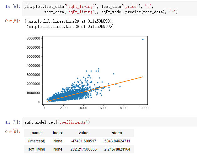
import graphlab
import matplotlib.pyplot as plt
%matplotlib inline

sales = gl.SFrame('data/home_data.gl/')

#下面这两行调用canvas进行网页可视化
#graphlab.canvas.set_target('ipynb')                            #设置为在ipynb界面显示
#sales.show(view="Scatter Plot", x="sqft_living", y="price")    #绘出房价和面积的散点图

train_data, test_data = sales.random_split(0.8, seed=0)

#一、构建单变量回归模型
sqft_model = graphlab.linear_regression.create(train_data, target='price', features=['sqft_living'])

#模型评估
print test_data['price'].mean()            #测试数据房价的均值    54W
print sqft_model.evaluate(test_data)    #sqft_model模型的最大误差 414W     和RMSE均方根误差 25.5W        差距还是有点多

plt.plot(test_data['sqft_living'], test_data['price'], '.',
         test_data['sqft_living'], sqft_model.predict(test_data), '-')

sqft_model.get('coefficients')            #模型系数


#二、构建多变量回归模型
my_features = ['bedrooms', 'bathrooms', 'sqft_living', 'sqft_lot', 'floors', 'zipcode']
#下面两行进行初步观察,看一下这些特征的数值分布
#sales[my_features].show()
#sales.show(view='BoxWhisker Plot', x='zipcode', y='price')
my_features_model = graphlab.linear_regression.create(train_data, target='price', features=my_features)
print my_features_model.evaluate(test_data)        #my_features_model模型的最大误差 353W     和RMSE均方根误差 17.8W


#模型应用
house1 = sales[sales['id'] == '5309101200']        #取出一个实例
sqft_model.predict(test_data)                    #测试集房价预测
my_features_model.predict(house1)                #对实例进行预测

二、分类模型——商品的情感分类
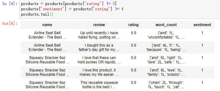
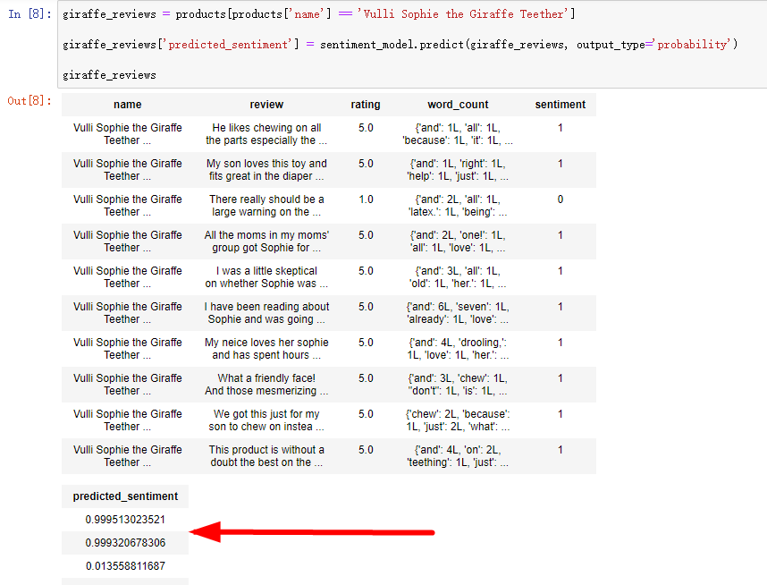
import graphlab

products = graphlab.SFrame('data/amazon_baby.gl/')    #读取商品的评价数据

#对于每个评价建立单词计数向量
products['word_count'] = graphlab.text_analytics.count_words(products['review'])

#下面这两行调用canvas进行网页可视化
#products['name'].show()
#products['rating'].show(view='Categorical')    #查看评分的分布

#定义正面和负面的标签    4/5分为正面,1/2分为负面,去掉中间的3分
products = products[products['rating'] != 3]
products['sentiment'] = products['rating'] >= 4

train_data, test_data = products.random_split(0.8, seed=0)

#训练情感分类器
sentiment_model = graphlab.logistic_classifier.create(train_data,
                                                      target='sentiment',
                                                      features=['word_count'],
                                                      validation_set=test_data)
#模型评估
sentiment_model.evaluate(test_data, metric='roc_curve')
sentiment_model.show(view='Evaluation')

#模型应用
giraffe_reviews = products[products['name'] == 'Vulli Sophie the Giraffe Teether']
giraffe_reviews['predicted_sentiment'] = sentiment_model.predict(giraffe_reviews, output_type='probability')      #输出类型设置为概率
giraffe_reviews = giraffe_reviews.sort('predicted_sentiment', ascending=False)                                    #评价排序

giraffe_reviews[0]['review']    #查看最棒的评价
giraffe_reviews[-1]['review']    #查看最差的评价

三、聚类模型——维基百科人物分类

假设词袋里有64篇文档,其中63篇都包含单词the,所以单词the的逆向文档频率为0。同理,单词Messi(梅西)的频率为4
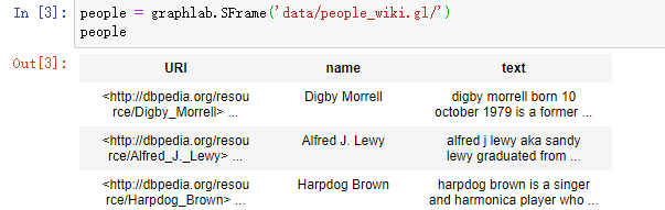
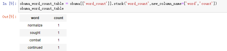
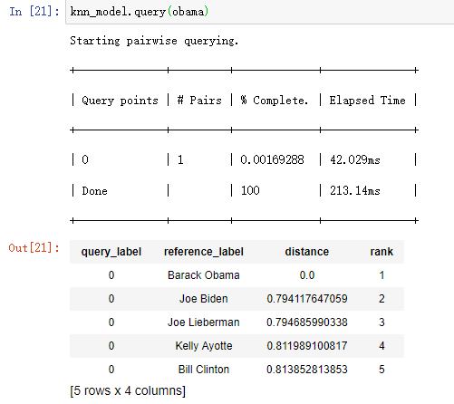
import graphlab

people = graphlab.SFrame('data/people_wiki.gl/')

#分析奥巴马
obama = people[people['name'] == 'Barack Obama']
obama['word_count'] = graphlab.text_analytics.count_words(obama['text'])                                #取得奥巴马文章中的单词计数
obama_word_count_table = obama[['word_count']].stack('word_count', new_column_name=['word', 'count'])    #将word_count分成word和count两列
obama_word_count_table.sort('count', ascending=False)    #查看奥巴马文档中出现最多的单词(即词频降序排列)

#计算语料库中的TF-IDF
people['word_count'] = graphlab.text_analytics.count_words(people['text'])
tfidf = graphlab.text_analytics.tf_idf(people['word_count'])
people['tfidf'] = tfidf            #people中构建新的特征tfidf

#检查奥巴马文章中的TF-IDF
obama = people[people['name'] == 'Barack Obama']                                                    #重新读入奥巴马数据,此时读入后带有tfidf字段(若不重新读入,下面句代码会报错)
obama[['tfidf']].stack('tfidf', new_column_name=['word', 'tfidf']).sort('tfidf', ascending=False)    #按照TF-IDF降序排列(并非单纯的词频排序哈)

#计算几个人之间的距离
clinton = people[people['name'] == 'Bill Clinton']
beckham = people[people['name'] == 'David Beckham']
print graphlab.distances.cosine(obama['tfidf'][0], clinton['tfidf'][0])    #奥巴马和克林顿的余弦距离为0.83
print graphlab.distances.cosine(obama['tfidf'][0], beckham['tfidf'][0])    #奥巴马和贝克汉姆的余弦距离为0.97        所以奥巴马和克林顿更“相似”

#构建文档检索的最近邻域模型
knn_model = graphlab.nearest_neighbors.create(people, features=['tfidf'], label='name')
print knn_model.query(obama)        #谁和奥巴马最接近
print knn_model.query(beckham)    #谁和贝克汉姆最接近

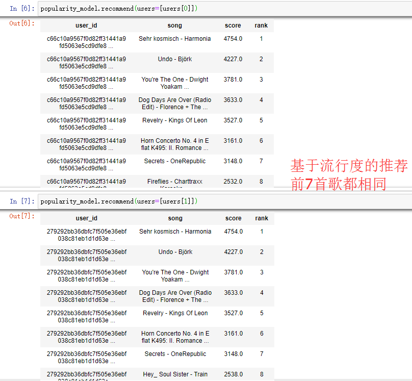
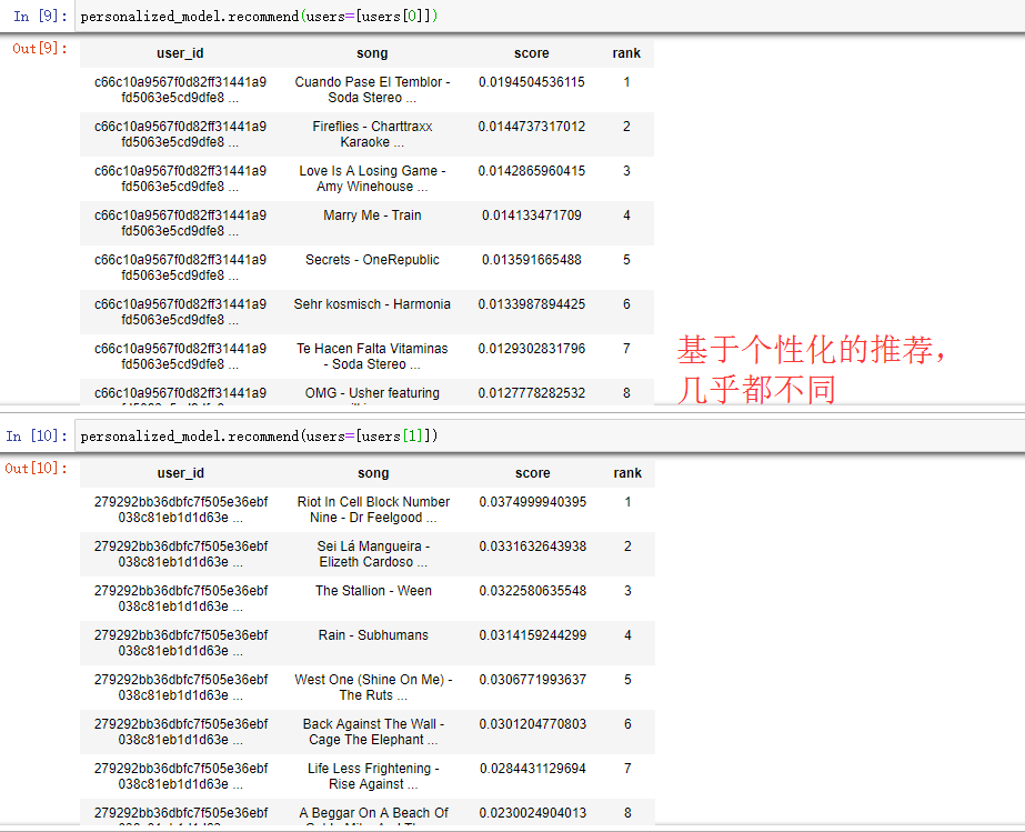
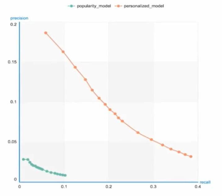
四、推荐系统——音乐推荐
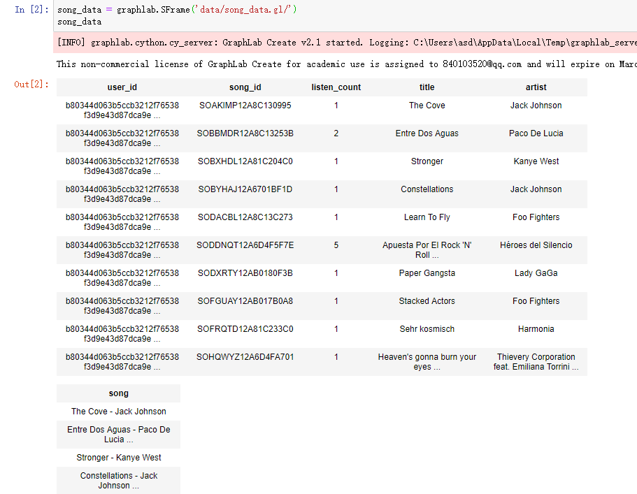
import graphlab

song_data = graphlab.SFrame('data/song_data.gl/')

#song_data['song'].show()                #展示数据集中最流行的音乐
print len(song_data)                     #111W条

users = song_data['user_id'].unique()    #用户去重
print len(users)                         #6.6W条,和歌曲数目不同(因为一个人可能听很多首歌)

train_data, test_data = song_data.random_split(0.8, seed=0)

#基于流行度的推荐系统
popularity_model = graphlab.popularity_recommender.create(train_data, user_id='user_id', item_id='song')
#对用户0和用户1的推荐,和最流行的音乐榜几乎一致
popularity_model.recommend(users=[users[0]])
popularity_model.recommend(users=[users[1]])


#基于个性化的推荐系统
personalized_model = graphlab.item_similarity_recommender.create(train_data, user_id='user_id', item_id='song')
#对于用户0和用户1的推荐大不相同
personalized_model.recommend(users=[users[0]])
personalized_model.recommend(users=[users[1]])

#推荐系统的比较
model_performance = graphlab.compare(test_data, [popularity_model, personalized_model], user_sample=0.05)
graphlab.show_comparison(model_performance, [popularity_model, personalized_model])
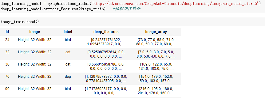
五、深度学习——图像检索系统
import graphlab

image_train = graphlab.SFrame('data/image_train_data/')

#下面两行运行很久,且报错
#deep_learning_model = graphlab.load_model('http://s3.amazonaws.com/GraphLab-Datasets/deeplearning/imagenet_model_iter45')        #导入深度学习模型
#deep_learning_model.extract_features(image_train)   #通过模型抽取image_train深度特征

#基于深度特征构建K近邻模型,从而进行图像检索
knn_model = graphlab.nearest_neighbors.create(image_train, features=['deep_features'], label='id')

#寻找猫的相似图像
cat = image_train[18:19]    #取出某只猫的图像,不妨给这只猫命名为tony
#cat['image'].show()
knn_model.query(cat)        #进行检索

#通过reference_label关联id得到images(即取出reference_label=id的图像)
def get_images_from_ids(query_result):
    return image_train.filter_by(query_result['reference_label'], 'id')

cat_neighbors = get_images_from_ids(knn_model.query(cat))    #通过上述函数得到这只tony猫的“邻居”
cat_neighbors['image'].show()


#寻找轿车的相似图像
car = image_train[8:9]
#car['image'].show()
get_images_from_ids(knn_model.query(car))['image'].show()


#构造一个lambda函数来寻找和显示最近的图像
show_neighbors = lambda i: get_images_from_ids(knn_model.query(image_train[i:i+1]))['image'].show()
show_neighbors(8)    #显示tony猫的“邻居”
show_neighbors(18)    #显示小轿车的“邻居”