statistical learning

统计学习

https://scikit-learn.org/stable/tutorial/statistical_inference/index.html

      数据量不停增加，增加了机器学习的重要性。

     机器学习可以处理 预测 分类 学习非标记的数据结构。

     统计学习使用机器学习技术，达成统计推断目标， 从数据中得出结论。

     统计学习的目的还是统计的目的， 在已有数据中得出结论。

Statistical learning

Machine learning is a technique with a growing importance, as the size of the datasets experimental sciences are facing is rapidly growing.

Problems it tackles range from building a prediction function linking different observations, to classifying observations, or learning the structure in an unlabeled dataset.

This tutorial will explore statistical learning, the use of machine learning techniques with the goal of statistical inference: drawing conclusions on the data at hand.

Scikit-learn is a Python module integrating classic machine learning algorithms in the tightly-knit world of scientific Python packages (NumPy, SciPy, matplotlib).

统计推断

https://en.wikipedia.org/wiki/Statistical_inference

      统计推断，使用数据分析工具， 规约属性的潜在数据分布。

     推断性统计分析，推断群体特性， 例如 测试假设， 得出估计。 统计假设了 观察到的数据仅仅是 更大群体中的一个子集。

    描述性统计， 则只关注观察到的数据， 不考虑其来自的群体效果。

Statistical inference is the process of using data analysis to deduce properties of an underlying distribution of probability.^[1]

Inferential statistical analysis infers properties of a population, for example by testing hypotheses and deriving estimates. It is assumed that the observed data set is sampled from a larger population.

Inferential statistics can be contrasted with descriptive statistics.

Descriptive statistics is solely concerned with properties of the observed data, and it does not rest on the assumption that the data come from a larger population.

In machine learning, the term inference is sometimes used instead to mean "make a prediction, by evaluating an already trained model";^[2] in this context deducing properties of the model is referred to as training or learning (rather than inference), and using a model for prediction is referred to as inference (instead of prediction); see also predictive inference.

Supervised learning

     https://scikit-learn.org/stable/tutorial/statistical_inference/supervised_learning.html#supervised-learning-predicting-an-output-variable-from-high-dimensional-observations

     监督性学习存在于 学习两个数据集之间的关联关系。

    观察到的数据X， 和外部数据y，即目标数据。

The problem solved in supervised learning

Supervised learning consists in learning the link between two datasets: the observed data X and an external variable y that we are trying to predict, usually called “target” or “labels”. Most often, y is a 1D array of length n_samples.

All supervised estimators in scikit-learn implement a fit(X, y) method to fit the model and a predict(X) method that, given unlabeled observations X, returns the predicted labels y.

   监督性学习分为 分类 和 回归。

  分类 问题 的 目标值为 离散型数据。

  回归 问题 的目标值为 连续型数据。

Vocabulary: classification and regression

If the prediction task is to classify the observations in a set of finite labels, in other words to “name” the objects observed, the task is said to be a classification task. On the other hand, if the goal is to predict a continuous target variable, it is said to be a regression task.

When doing classification in scikit-learn, y is a vector of integers or strings.

Note: See the Introduction to machine learning with scikit-learn Tutorial for a quick run-through on the basic machine learning vocabulary used within scikit-learn.

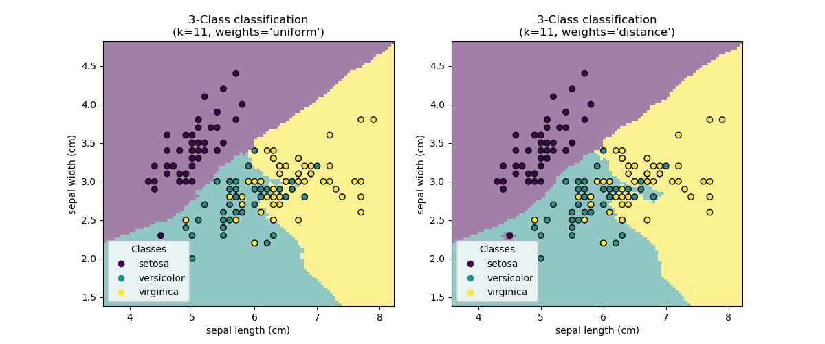
k-Nearest neighbors classifier

https://scikit-learn.org/stable/tutorial/statistical_inference/supervised_learning.html#k-nearest-neighbors-classifier

      最简单的分类是最近邻分类， 给出训练集合， 在训练集合中， 查找特征向量距离最近的数据， 将新数据的类别定位找到数据的类别。

The simplest possible classifier is the nearest neighbor: given a new observation X_test, find in the training set (i.e. the data used to train the estimator) the observation with the closest feature vector. (Please see the Nearest Neighbors section of the online Scikit-learn documentation for more information about this type of classifier.)

      一般在训练集合上训练模型，在测试数据上评价模型。

Training set and testing set

While experimenting with any learning algorithm, it is important not to test the prediction of an estimator on the data used to fit the estimator as this would not be evaluating the performance of the estimator on new data. This is why datasets are often split into train and test data.

KNN (k nearest neighbors) classification example:

>>>

>>> # Split iris data in train and test data
>>> # A random permutation, to split the data randomly
>>> np.random.seed(0)
>>> indices = np.random.permutation(len(iris_X))
>>> iris_X_train = iris_X[indices[:-10]]
>>> iris_y_train = iris_y[indices[:-10]]
>>> iris_X_test = iris_X[indices[-10:]]
>>> iris_y_test = iris_y[indices[-10:]]
>>> # Create and fit a nearest-neighbor classifier
>>> from sklearn.neighbors import KNeighborsClassifier
>>> knn = KNeighborsClassifier()
>>> knn.fit(iris_X_train, iris_y_train)
KNeighborsClassifier()
>>> knn.predict(iris_X_test)
array([1, 2, 1, 0, 0, 0, 2, 1, 2, 0])
>>> iris_y_test
array([1, 1, 1, 0, 0, 0, 2, 1, 2, 0])

The curse of dimensionality （维数灾难）

    特征很多的情况下， 特征维数就会很多， 机器学习基于距离的学习方法，区分度将会变得很小， 当维数增加时。

     维数灾难是机器学习需要解决的核心问题。

For example, if each point is just a single number (8 bytes), then an effective -NN estimator in a paltry

dimensions would require more training data than the current estimated size of the entire internet (±1000 Exabytes or so).

This is called the curse of dimensionality and is a core problem that machine learning addresses.

https://www.zhihu.com/question/27836140

      从样本覆盖度量角度更好理解。

在样本量一定的情况下，维度越高，样本在空间中的分布越呈现稀疏性。

这很容易理解。假设随机变量服从均匀分布，如果一维空间（即数轴上的某一区间）需要N个样本才能完全覆盖，那么当二维空间下还是N个样本时，覆盖度就有所下降。随着维度的增加，覆盖度指数级下降。

这种分布的稀疏性带来2个不好的影响：

1、 模型参数难以正确估计（例如：样本不够时，得出的决策边界往往是过拟合的）。假设均匀分布下，一维空间（即数轴上的某一区间）需要N个样本才能完全覆盖，那么二维均匀分布下就需要N^2个样本才能完全覆盖,三维N^3个,依次类推。因此，随着维度的增加，理论上需要指数增长的样本数量覆盖到整个样本空间上时，才能保证模型能有效的估计参数。而对于那些具有非线性决策边界的分类器（如：神经网络，决策树，KNN）来说，如果样本不够多时，往往很容易过拟合。

2、 样本分布位于中心附近的概率，随着维度的增加，越来越低；而样本处在边缘的概率，则越来越高。通常来讲，样本的特征位于边缘时，比位于中心区域附近更难分类，因为边缘样本的特征取值范围变化太大。想象二维空间下的两个同心圆，假设r1=0.5，r2=1，那么面积之比为1/4；如果半径不变，在三维空间中，体积之比变成1/8；到了8维空间下，超球体的体积之比为1/256，仅仅占到2%。当维数趋于无穷时，位于中心附近的概率趋于0。这种情况下，一些度量相异性的距离指标（如：欧式距离）效果会大大折扣，从而导致一些基于这些指标的分类器在高维度的时候表现不好。

Diabetes dataset

     糖尿病数据集是典型的回归性数据集合。

The diabetes dataset consists of 10 physiological variables (age, sex, weight, blood pressure) measure on 442 patients, and an indication of disease progression after one year:

>>>

>>> diabetes_X, diabetes_y = datasets.load_diabetes(return_X_y=True)
>>> diabetes_X_train = diabetes_X[:-20]
>>> diabetes_X_test  = diabetes_X[-20:]
>>> diabetes_y_train = diabetes_y[:-20]
>>> diabetes_y_test  = diabetes_y[-20:]

The task at hand is to predict disease progression from physiological variables.

Linear regression

https://scikit-learn.org/stable/tutorial/statistical_inference/supervised_learning.html#linear-regression

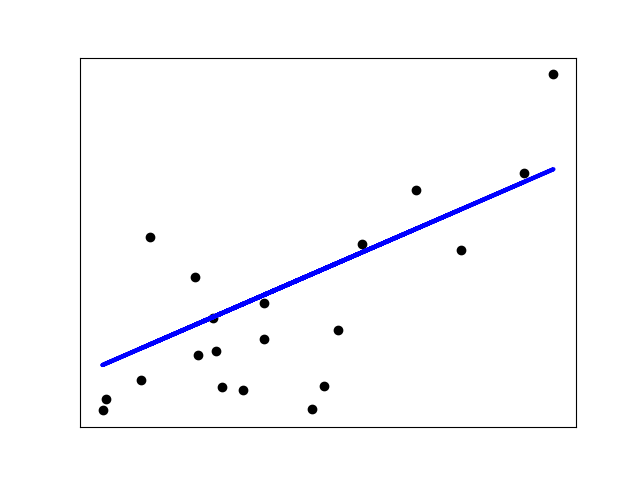
     线性模型， 是最简单的回归模型， 其使用直线来拟合数据。

LinearRegression, in its simplest form, fits a linear model to the data set by adjusting a set of parameters in order to make the sum of the squared residuals of the model as small as possible.

Linear models:

• : Observation noise

>>

>>> from sklearn import linear_model
>>> regr = linear_model.LinearRegression()
>>> regr.fit(diabetes_X_train, diabetes_y_train)
LinearRegression()
>>> print(regr.coef_)
[   0.30349955 -237.63931533  510.53060544  327.73698041 -814.13170937
  492.81458798  102.84845219  184.60648906  743.51961675   76.09517222]


>>> # The mean square error
>>> np.mean((regr.predict(diabetes_X_test) - diabetes_y_test)**2)
2004.56760268...

>>> # Explained variance score: 1 is perfect prediction
>>> # and 0 means that there is no linear relationship
>>> # between X and y.
>>> regr.score(diabetes_X_test, diabetes_y_test)
0.5850753022690...

缺点

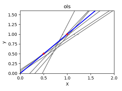
     对于少量噪音数据， 会造成拟合曲线的巨大偏差。

If there are few data points per dimension, noise in the observations induces high variance:

>>>

>>> X = np.c_[ .5, 1].T
>>> y = [.5, 1]
>>> test = np.c_[ 0, 2].T
>>> regr = linear_model.LinearRegression()

>>> import matplotlib.pyplot as plt 
>>> plt.figure() 

>>> np.random.seed(0)
>>> for _ in range(6): 
...     this_X = .1 * np.random.normal(size=(2, 1)) + X
...     regr.fit(this_X, y)
...     plt.plot(test, regr.predict(test)) 
...     plt.scatter(this_X, y, s=3)  

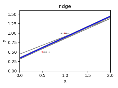
岭回归

解决线性模型缺点的方法。

A solution in high-dimensional statistical learning is to shrink the regression coefficients to zero: any two randomly chosen set of observations are likely to be uncorrelated. This is called Ridge regression:

>>>

>>> regr = linear_model.Ridge(alpha=.1)

>>> plt.figure() 

>>> np.random.seed(0)
>>> for _ in range(6): 
...     this_X = .1 * np.random.normal(size=(2, 1)) + X
...     regr.fit(this_X, y)
...     plt.plot(test, regr.predict(test)) 
...     plt.scatter(this_X, y, s=3) 

This is an example of bias/variance tradeoff: the larger the ridge alpha parameter, the higher the bias and the lower the variance.

     参数alpha的选择，是对偏差和方差一个折中。

We can choose alpha to minimize left out error, this time using the diabetes dataset rather than our synthetic data:

>>>

>>> alphas = np.logspace(-4, -1, 6)
>>> print([regr.set_params(alpha=alpha)
...            .fit(diabetes_X_train, diabetes_y_train)
...            .score(diabetes_X_test, diabetes_y_test)
...        for alpha in alphas])
[0.5851110683883..., 0.5852073015444..., 0.5854677540698...,
 0.5855512036503..., 0.5830717085554..., 0.57058999437...]

Note

Capturing in the fitted parameters noise that prevents the model to generalize to new data is called overfitting. The bias introduced by the ridge regression is called a regularization.

Ridge原理

https://scikit-learn.org/stable/modules/generated/sklearn.linear_model.Ridge.html#sklearn.linear_model.Ridge

     岭回归之所以能够抑制噪音点的影响， 是因为， 对于线性模型对应的 系数 应用了惩罚项。

    这里的系数可以理解为 集合上的 斜率。

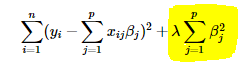
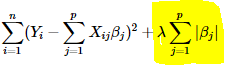
    在目标函数中， 添加 系数矩阵的 L2正则 惩罚项。

    在计算过程中， 为了使得目标函数最小 系数矩阵中的 系数， 在惩罚项的帮助下， 会变得更小。

Linear least squares with l2 regularization.

Minimizes the objective function:

||y - Xw||^2_2 + alpha * ||w||^2_2

This model solves a regression model where the loss function is the linear least squares function and regularization is given by the l2-norm.

Also known as Ridge Regression or Tikhonov regularization.

This estimator has built-in support for multi-variate regression (i.e., when y is a 2d-array of shape (n_samples, n_targets)).

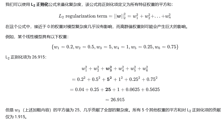
L1 and L2 Regularization Methods

https://towardsdatascience.com/l1-and-l2-regularization-methods-ce25e7fc831c

A regression model that uses L1 regularization technique is called Lasso Regression and model which uses L2 is called Ridge Regression.

岭回归

Ridge regression adds “squared magnitude” of coefficient as penalty term to the loss function. Here the highlighted part represents L2 regularization element.

Lasso回归

Lasso Regression (Least Absolute Shrinkage and Selection Operator) adds “absolute value of magnitude” of coefficient as penalty term to the loss function.

     lasso回归更加狠，会将一些系数惩罚为 0.

The key difference between these techniques is that Lasso shrinks the less important feature’s coefficient to zero thus, removing some feature altogether. So, this works well for feature selection in case we have a huge number of features.

https://developers.google.com/machine-learning/crash-course/regularization-for-simplicity/l2-regularization

Sparsity -- 特征稀疏性

     例如 维度2 特征提供的信息非常少， 完全可以忽略。

    则使用lasso回归更加合适。牺牲掉那个维度的特征。减少维数灾难。

    这个符合 奥卡姆剃刀原则。

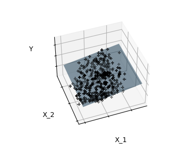
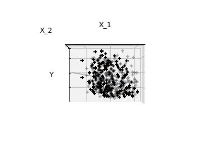
Fitting only features 1 and 2

Note

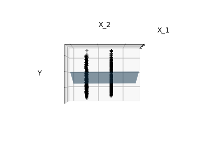
A representation of the full diabetes dataset would involve 11 dimensions (10 feature dimensions and one of the target variable). It is hard to develop an intuition on such representation, but it may be useful to keep in mind that it would be a fairly empty space.

We can see that, although feature 2 has a strong coefficient on the full model, it conveys little information on y when considered with feature 1.

To improve the conditioning of the problem (i.e. mitigating the The curse of dimensionality), it would be interesting to select only the informative features and set non-informative ones, like feature 2 to 0. Ridge regression will decrease their contribution, but not set them to zero. Another penalization approach, called Lasso (least absolute shrinkage and selection operator), can set some coefficients to zero. Such methods are called sparse method and sparsity can be seen as an application of Occam’s razor: prefer simpler models.

>>> regr = linear_model.Lasso()
>>> scores = [regr.set_params(alpha=alpha)
...               .fit(diabetes_X_train, diabetes_y_train)
...               .score(diabetes_X_test, diabetes_y_test)
...           for alpha in alphas]
>>> best_alpha = alphas[scores.index(max(scores))]
>>> regr.alpha = best_alpha
>>> regr.fit(diabetes_X_train, diabetes_y_train)
Lasso(alpha=0.025118864315095794)
>>> print(regr.coef_)
[   0.         -212.437...  517.194...  313.779... -160.830...
   -0.         -187.195...   69.382...  508.660...   71.842...]

奥卡姆剃刀

https://www.zhihu.com/topic/19659363/intro

      如无必要，不要增加复杂性。 ----- “plurality should not be posited without necessity.”

奥卡姆剃刀（英语：Occam's Razor, Ockham's Razor），又称“奥坎的剃刀”，拉丁文为lex parsimoniae，意思是简约之法则，是由14世纪逻辑学 家、圣方济各会 修士 奥卡姆的威廉 （William of Occam，约1287年至1347年，奥卡姆（Ockham）位于英格兰 的萨里郡 ）提出的一个解决问题的法则，他在《箴言书注》2卷15题说“切勿浪费较多东西，去做‘用较少的东西，同样可以做好的事情’。”换一种说法，如果关于同一个问题有许多种理论，每一种都能作出同样准确的预言，那么应该挑选其中使用假定最少的。尽管越复杂的方法通常能作出越好的预言，但是在不考虑预言能力的情况下，前提假设越少越好。

https://www.britannica.com/topic/Occams-razor

“plurality should not be posited without necessity.”

Occam’s razor, also spelled Ockham’s razor, also called law of economy or law of parsimony, principle stated by the Scholastic philosopher William of Ockham (1285–1347/49) that pluralitas non est ponenda sine necessitate,

“plurality should not be posited without necessity.”

The principle gives precedence to simplicity: of two competing theories, the simpler explanation of an entity is to be preferred. The principle is also expressed as “Entities are not to be multiplied beyond necessity.”

William of Ockham

William of Ockham.

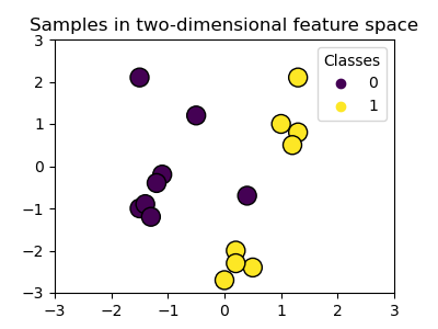
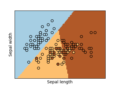
Classification

https://scikit-learn.org/stable/tutorial/statistical_inference/supervised_learning.html#classification

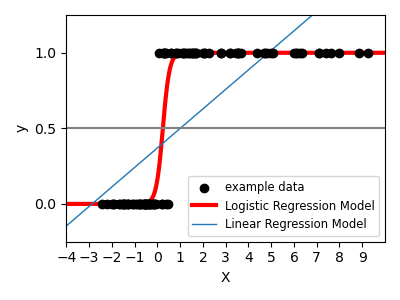
      线性回归是对噪音敏感。

      逻辑回归分类，使用过滤函数 logistic函数 将噪音降低。

For classification, as in the labeling iris task, linear regression is not the right approach as it will give too much weight to data far from the decision frontier.

A linear approach is to fit a sigmoid function or logistic function:

 

>>>

>>> log = linear_model.LogisticRegression(C=1e5)
>>> log.fit(iris_X_train, iris_y_train)
LogisticRegression(C=100000.0)

This is known as LogisticRegression.

     逻辑回归 也 可以设置  L1 或者 L2 惩罚项。

Shrinkage and sparsity with logistic regression

The C parameter controls the amount of regularization in the LogisticRegression object: a large value for C results in less regularization. penalty="l2" gives Shrinkage (i.e. non-sparse coefficients), while penalty="l1" gives Sparsity

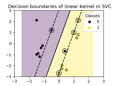
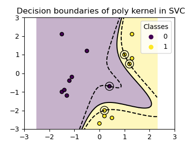
Support vector machines (SVMs)

https://scikit-learn.org/stable/tutorial/statistical_inference/supervised_learning.html#support-vector-machines-svms

Linear SVMs

      支持向量机， 可以支持分类和回归。

Support Vector Machines belong to the discriminant model family: they try to find a combination of samples to build a plane maximizing the margin between the two classes. Regularization is set by the C parameter: a small value for C means the margin is calculated using many or all of the observations around the separating line (more regularization); a large value for C means the margin is calculated on observations close to the separating line (less regularization).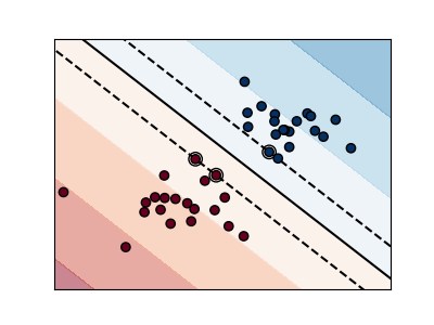

Unregularized SVM

Regularized SVM (default)

     根据核函数的选择不同， 其支持的分类或者回归能力不同。

Using kernels

Classes are not always linearly separable in feature space. The solution is to build a decision function that is not linear but may be polynomial instead. This is done using the kernel trick that can be seen as creating a decision energy by positioning kernels on observations:

Linear kernel

>>>

>>> svc = svm.SVC(kernel='linear')

Polynomial kernel

>>>

>>> svc = svm.SVC(kernel='poly',
...               degree=3)
>>> # degree: polynomial degree

RBF kernel (Radial Basis Function)

>>>

>>> svc = svm.SVC(kernel='rbf')
>>> # gamma: inverse of size of
>>> # radial kernel