Kmeans作为机器学习中入门级算法,涉及到计算距离算法的选择,聚类中心个数的选择。下面就简单介绍一下在R语言中是怎么解决这两个问题的。
参考Unsupervised Learning with R
> Iris<-iris
> #K mean
> set.seed(123)
> KM.Iris<-kmeans(Iris[1:4],3,iter.max=1000,algorithm = c("Forgy"))
> KM.Iris$size
[1] 50 39 61
> KM.Iris$centers  #聚类的3个中心
  Sepal.Length Sepal.Width Petal.Length Petal.Width
1     5.006000    3.428000     1.462000    0.246000
2     6.853846    3.076923     5.715385    2.053846
3     5.883607    2.740984     4.388525    1.434426
> str(KM.Iris)
List of 9
 $ cluster     : int [1:150] 1 1 1 1 1 1 1 1 1 1 ...
 $ centers     : num [1:3, 1:4] 5.01 6.85 5.88 3.43 3.08 ...
  ..- attr(*, "dimnames")=List of 2
  .. ..$ : chr [1:3] "1" "2" "3"
  .. ..$ : chr [1:4] "Sepal.Length" "Sepal.Width" "Petal.Length" "Petal.Width"
 $ totss       : num 681
 $ withinss    : num [1:3] 15.2 25.4 38.3
 $ tot.withinss: num 78.9
 $ betweenss   : num 603
 $ size        : int [1:3] 50 39 61
 $ iter        : int 2
 $ ifault      : NULL
 - attr(*, "class")= chr "kmeans"
> table(Iris$Species,KM.Iris$cluster)
1 2 3
setosa 50 0 0
versicolor 0 3 47
virginica 0 36 14
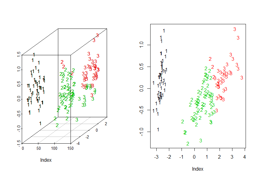
> Iris.dist<-dist(Iris[1:4])
> Iris.mds<-cmdscale(Iris.dist)
关于cmdscale,classical multidimensional scaling of a data matrix,也被成为是principal coordinates analysis
> par(mfrow=c(1,2))
> #3D
> library("scatterplot3d")
> chars<-c("1","2","3")[as.integer(iris$Species)]
> g3d<-scatterplot3d(Iris.mds,pch=chars)
> g3d$points3d(iris.mds,col=KM.Iris$cluster,pch=chars)
> #2D
> plot(Iris.mds,col=KM.Iris$cluster,pch=chars,xlab="Index",ylab= "Y")
> KM.Iris[1]
$cluster
[1] 1 1 1 1 1 1 1 1 1 1 1 1 1 1 1 1 1 1 1 1 1 1 1 1 1 1 1 1 1 1 1 1 1 1 1 1 1 1 1 1 1 1 1 1 1 1 1 1 1 1 2 3 2 3 3 3 3 3
[59] 3 3 3 3 3 3 3 3 3 3 3 3 3 3 3 3 3 3 3 2 3 3 3 3 3 3 3 3 3 3 3 3 3 3 3 3 3 3 3 3 3 3 2 3 2 2 2 2 3 2 2 2 2 2 2 3 3 2
[117] 2 2 2 3 2 3 2 3 2 2 3 3 2 2 2 2 2 3 2 2 2 2 3 2 2 2 3 2 2 2 3 2 2 3
> Iris.cluster<-cbind(Iris,KM.Iris$cluster)
> head(Iris.cluster)
Sepal.Length Sepal.Width Petal.Length Petal.Width Species KM.Iris$cluster
1 5.1 3.5 1.4 0.2 setosa 1
2 4.9 3.0 1.4 0.2 setosa 1
3 4.7 3.2 1.3 0.2 setosa 1
4 4.6 3.1 1.5 0.2 setosa 1
5 5.0 3.6 1.4 0.2 setosa 1
6 5.4 3.9 1.7 0.4 setosa 1
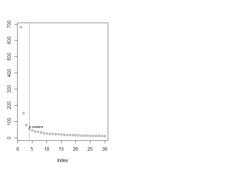
> # 下面寻找最佳簇数目
> # 30 Kmeans loop
> InerIC<-rep(0,30);InerIC
[1] 0 0 0 0 0 0 0 0 0 0 0 0 0 0 0 0 0 0 0 0 0 0 0 0 0 0 0 0 0 0
> for (k in 1:30){
+ set.seed(123)
+ groups=kmeans(Iris[1:4],k)
+ InerIC[k]<-groups$tot.withinss
+ }
> InerIC
[1] 681.37060 152.34795 78.85144 57.26562 46.46117 39.05498 37.34900 32.58266 28.46897 26.32133 24.92591
[12] 23.52298 23.33464 21.83167 20.04231 19.21720 17.82750 17.35801 16.69589 15.74660 14.53898 13.61800
[23] 13.38004 12.81350 12.37310 12.02532 11.72245 11.55765 11.04824 10.56507
> groups
K-means clustering with 30 clusters of sizes 5, 4, 1, 5, 7, 5, 9, 3, 4, 2, 3, 4, 3, 7, 4, 5, 8, 5, 4, 3, 9, 1, 6, 4, 4, 8, 1, 3, 10, 13
Cluster means:
Sepal.Length Sepal.Width Petal.Length Petal.Width
1 4.940000 3.400000 1.680000 0.3800000
2 7.675000 2.850000 6.575000 2.1750000
3 5.000000 2.000000 3.500000 1.0000000
4 7.240000 2.980000 6.020000 1.8400000
5 6.442857 2.828571 5.557143 1.9142857
6 4.580000 3.320000 1.280000 0.2200000
7 6.722222 3.000000 4.677778 1.4555556
8 6.233333 3.300000 4.566667 1.5666667
9 6.150000 2.900000 4.200000 1.3500000
10 5.400000 2.800000 3.750000 1.3500000
11 6.133333 2.700000 5.266667 1.5000000
12 6.075000 2.900000 4.625000 1.3750000
13 5.000000 2.400000 3.200000 1.0333333
14 6.671429 3.085714 5.257143 2.1571429
15 4.400000 2.800000 1.275000 0.2000000
16 5.740000 2.700000 5.040000 2.0400000
17 5.212500 3.812500 1.587500 0.2750000
18 5.620000 4.060000 1.420000 0.3000000
19 5.975000 3.050000 4.900000 1.8000000
20 7.600000 3.733333 6.400000 2.2333333
21 6.566667 3.244444 5.711111 2.3333333
22 4.900000 2.500000 4.500000 1.7000000
23 5.550000 2.450000 3.816667 1.1333333
24 6.275000 2.625000 4.900000 1.7500000
25 5.775000 2.700000 4.025000 1.1750000
26 5.600000 2.875000 4.325000 1.3250000
27 6.000000 2.200000 4.000000 1.0000000
28 6.166667 2.233333 4.633333 1.4333333
29 4.840000 3.080000 1.470000 0.1900000
30 5.146154 3.461538 1.438462 0.2230769
Clustering vector:
[1] 30 29 6 29 30 17 6 30 15 29 17 1 29 15 18 18 18 30 18 17 30 17 6 1 1 29 1 30 30 29 29 30 17 18 29 29 30 30 15
[40] 30 30 15 6 1 17 29 17 6 17 30 7 8 7 23 7 26 8 13 7 10 3 9 27 12 10 7 26 25 28 23 19 9 24 12 9 7 7 7
[79] 12 23 23 23 25 11 26 8 7 28 26 23 26 12 25 13 26 26 26 9 13 25 21 16 4 5 21 2 22 4 5 20 14 5 14 16 16 14 5
[118] 20 2 28 21 16 2 24 21 4 24 19 5 4 4 20 5 11 11 2 21 5 19 14 21 14 16 21 21 14 24 14 21 19
Within cluster sum of squares by cluster:
[1] 0.2880000 0.5325000 0.0000000 0.4200000 0.6371429 0.2920000 0.7933333 0.1400000 0.2400000 0.1500000 0.2533333
[12] 0.1025000 0.1066667 0.5571429 0.4275000 0.2960000 0.5012500 0.5280000 0.1175000 0.5933333 1.0311111 0.0000000
[23] 0.3716667 0.1850000 0.1025000 0.5450000 0.0000000 0.2866667 0.3700000 0.6969231
(between_SS / total_SS = 98.4 %)
Available components:
[1] "cluster" "centers" "totss" "withinss" "tot.withinss" "betweenss" "size"
[8] "iter" "ifault"
> plot(InerIC,col = "black",lty =3)
There were 18 warnings (use warnings() to see them)
> abline(v=4,col="black",lty=3)
> text (4,60,"4 clusters",col="black",adj = c(0,-0.1),cex=0.7)
> library(NbClust)
> data<-Iris[,-5]
> head(data)
  Sepal.Length Sepal.Width Petal.Length Petal.Width
1          5.1         3.5          1.4         0.2
2          4.9         3.0          1.4         0.2
3          4.7         3.2          1.3         0.2
4          4.6         3.1          1.5         0.2
5          5.0         3.6          1.4         0.2
6          5.4         3.9          1.7         0.4
> best<-NbClust(data,diss=NULL,distance ="euclidean",min.nc=2, max.nc=15, method = "complete",index = "alllong")

*** : The Hubert index is a graphical method of determining the number of clusters.
                In the plot of Hubert index, we seek a significant knee that corresponds to a
                significant increase of the value of the measure i.e the significant peak in Hubert
                index second differences plot.
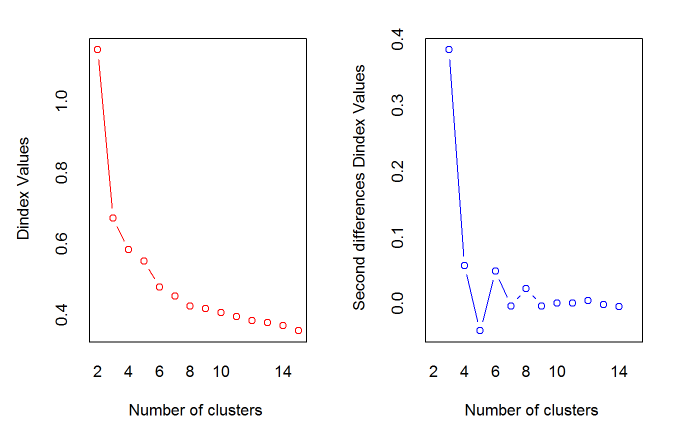
*** : The D index is a graphical method of determining the number of clusters.
In the plot of D index, we seek a significant knee (the significant peak in Dindex
second differences plot) that corresponds to a significant increase of the value of
the measure.
*******************************************************************
* Among all indices:
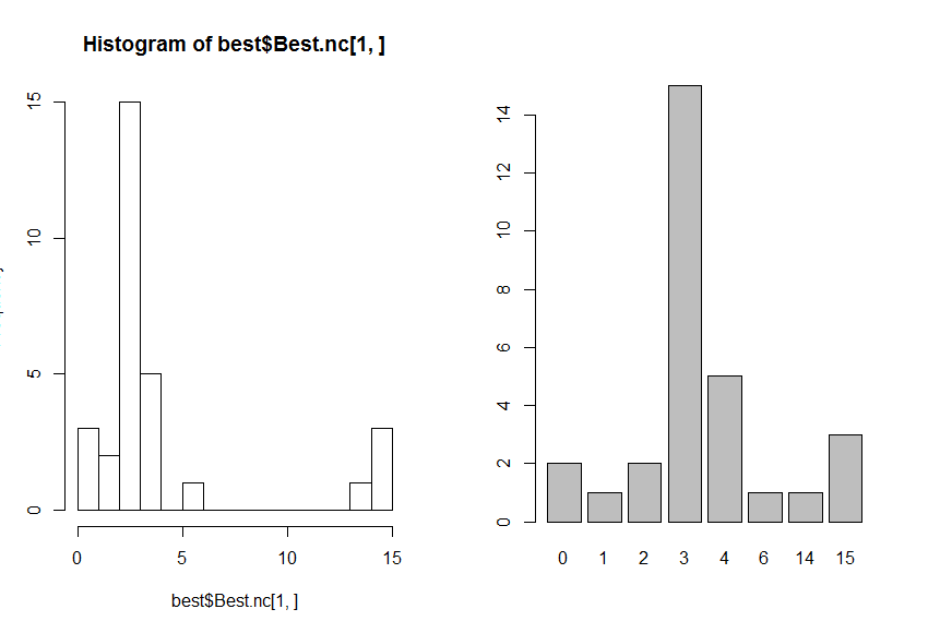
* 2 proposed 2 as the best number of clusters
* 15 proposed 3 as the best number of clusters
* 5 proposed 4 as the best number of clusters
* 1 proposed 6 as the best number of clusters
* 1 proposed 14 as the best number of clusters
* 3 proposed 15 as the best number of clusters
***** Conclusion *****
* According to the majority rule, the best number of clusters is 3
*******************************************************************
> table(names(best$Best.nc[1,]),best$Best.nc[1,])
0 1 2 3 4 6 14 15
Ball 0 0 0 1 0 0 0 0
Beale 0 0 0 1 0 0 0 0
CCC 0 0 0 1 0 0 0 0
CH 0 0 0 0 1 0 0 0
Cindex 0 0 0 1 0 0 0 0
DB 0 0 0 1 0 0 0 0
Dindex 1 0 0 0 0 0 0 0
Duda 0 0 0 0 1 0 0 0
Dunn 0 0 0 0 0 0 0 1
Frey 0 1 0 0 0 0 0 0
Friedman 0 0 0 0 1 0 0 0
Gamma 0 0 0 0 0 0 1 0
Gap 0 0 0 1 0 0 0 0
Gplus 0 0 0 0 0 0 0 1
Hartigan 0 0 0 1 0 0 0 0
Hubert 1 0 0 0 0 0 0 0
KL 0 0 0 0 1 0 0 0
Marriot 0 0 0 1 0 0 0 0
McClain 0 0 1 0 0 0 0 0
PseudoT2 0 0 0 0 1 0 0 0
PtBiserial 0 0 0 1 0 0 0 0
Ratkowsky 0 0 0 1 0 0 0 0
Rubin 0 0 0 0 0 1 0 0
Scott 0 0 0 1 0 0 0 0
SDbw 0 0 0 0 0 0 0 1
SDindex 0 0 0 1 0 0 0 0
Silhouette 0 0 1 0 0 0 0 0
Tau 0 0 0 1 0 0 0 0
TraceW 0 0 0 1 0 0 0 0
TrCovW 0 0 0 1 0 0 0 0
> hist(best$Best.nc[1,],breaks = max(na.omit(best$Best.nc[1,])))
> barplot(table(best$Best.nc[1,]))
> # 选择最佳聚类算法algorithm
> Hartigan <-0
> Lloyd <- 0
> Forgy <- 0
> MacQueen <- 0
> set.seed(123)
> # 做500次Kmeans计算,3个聚类中心,每次计算,每种算法迭代最多1000次
> for (i in 1:500){
+ KM<-kmeans(Iris[1:4],3,iter.max = 1000,algorithm = "Hartigan-Wong")
+ Hartigan <- Hartigan + KM$betweenss
+ KM<-kmeans(Iris[1:4],3,iter.max = 1000,algorithm = "Lloyd")
+ Lloyd <- Lloyd + KM$betweenss
+ KM<-kmeans(Iris[1:4],3,iter.max = 1000,algorithm = "Forgy")
+ Forgy <- Forgy + KM$betweenss
+ KM<-kmeans(Iris[1:4],3,iter.max = 1000,algorithm = "MacQueen")
+ MacQueen <- MacQueen + KM$betweenss
+ }
> # 输出结果
> Methods <- c("Hartigan","Lloyd","Forgy","MacQueen")
> Results <- as.data.frame(round(c(Hartigan,Lloyd,Forgy,MacQueen)/500,2))
> Results <- cbind(Methods,Results)
> names(Results) <- c("Method","Betweenss")
> Results
Method Betweenss
1 Hartigan 590.76
2 Lloyd 589.38
3 Forgy 590.63
4 MacQueen 590.05
> #作图
> par(mfrow =c(1,1))
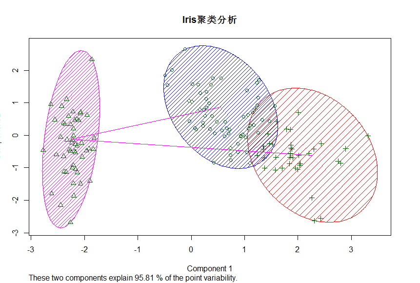
> KM<-kmeans(Iris[1:4],3,iter.max = 1000,algorithm = "Hartigan-Wong")
> library(cluster)
> clusplot(Iris[1:4],KM$cluster,color = T,shade = T,lables=2,lines = 1,main = "Iris聚类分析")
There were 50 or more warnings (use warnings() to see the first 50)
> library(HSAUR)
There were 50 or more warnings (use warnings() to see the first 50)
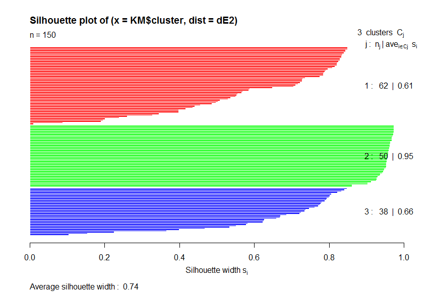
> diss <- daisy(Iris[1:4])
> dE2 <- diss^2
> obj <-silhouette(KM$cluster,dE2)
> plot(obj,col=c("red","green","blue"))