《DSP using MATLAB》示例 Example 10.1

坚持到第10章了，继续努力！

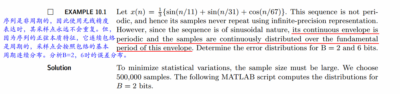
代码：

%% ------------------------------------------------------------------------
%%            Output Info about this m-file
fprintf('
***********************************************************
');
fprintf('        <DSP using MATLAB> Exameple 10.1 

');

time_stamp = datestr(now, 31);
[wkd1, wkd2] = weekday(today, 'long');
fprintf('      Now is %20s, and it is %7s  

', time_stamp, wkd2);
%% ------------------------------------------------------------------------

clear; close all;

% Example parameters
B = 2; N = 500000; n = [1:N];
xn = (1/3)*(sin(n/11) + sin(n/31) + cos(n/67)); clear n;

% Quantization error analysis
[H1, H2, Q, estat] = StatModelR(xn, B, N);          % Compute histograms
H1max = max(H1); H1min = min(H1);                   % Max and Min of H1
H2max = max(H2); H2min = min(H2);                   % Max and Min of H2



Hf1 = figure('units', 'inches', 'position', [1, 1, 8, 6], ...
	'paperunits', 'inches', 'paperposition', [0, 0, 6, 4], ...
	'NumberTitle', 'off', 'Name', 'Exameple 10.1a');
set(gcf,'Color','white'); 
TF = 10;
title('Normalized error e1 and e2'); 
subplot(2, 1, 1); 
bar(Q, H1); axis([-0.5, 0.5, -0.001, 4/128]); grid on;

xlabel('Normalized error e1'); ylabel('Distribution of e1 ', 'vertical', 'baseline'); 
set(gca, 'YTickMode', 'manual', 'YTick', [0, [1:1:4]/128] );
text(-0.45, 0.030, sprintf('SAMPLE SIZE N = %d', N));
text(-0.45, 0.025, sprintf(' ROUNDED TO B = %d BITS', B));
text(-0.45, 0.020, sprintf('                   MEAN  =  %.4e', estat(1)));
text(0.10, 0.030, sprintf('MIN PROB BAR HEIGHT =  %f', H1min)) ;
text(0.10, 0.025, sprintf('MAX PROB BAR HEIGHT = %f', H1max)) ;
text(0.10, 0.020, sprintf('                                 SIGMA = %f', estat(2))) ;


subplot(2, 1, 2);
bar(Q, H2); axis([-0.5, 0.5, -0.001, 4/128]); grid on;
%title('Normalized error e2'); 
xlabel('Normalized error e2'); ylabel('Distribution of e2', 'vertical', 'baseline'); 
set(gca, 'YTickMode', 'manual', 'YTick', [0, 1:1:4]/128 );
text(-0.45, 0.030, sprintf('SAMPLE SIZE N = %d', N));
text(-0.45, 0.025, sprintf(' ROUNDED TO B = %d BITS', B));
text(-0.45, 0.020, sprintf('                   MEAN  =  %.4e', estat(3)));
text(0.10, 0.030, sprintf('MIN PROB BAR HEIGHT =  %f', H2min)) ;
text(0.10, 0.025, sprintf('MAX PROB BAR HEIGHT = %f', H2max)) ;
text(0.10, 0.020, sprintf('                                 SIGMA = %f', estat(4))) ;

%% ---------------------------------------------------------------------
%%      B = 6 
%% ---------------------------------------------------------------------
% Example parameters
B = 6; N = 500000; n = [1:N];
xn = (1/3)*(sin(n/11) + sin(n/31) + cos(n/67)); clear n;

% Quantization error analysis
[H1, H2, Q, estat] = StatModelR(xn, B, N);          % Compute histograms
H1max = max(H1); H1min = min(H1);                   % Max and Min of H1
H2max = max(H2); H2min = min(H2);                   % Max and Min of H2



Hf2 = figure('units', 'inches', 'position', [1, 1, 8, 6], ...
	'paperunits', 'inches', 'paperposition', [0, 0, 6, 4], ...
	'NumberTitle', 'off', 'Name', 'Exameple 10.1b');
set(gcf,'Color','white'); 
TF = 10;

subplot(2, 1, 1); 
bar(Q, H1); axis([-0.5, 0.5, -0.001, 4/128]); grid on;
title('Normalized error e1'); ylabel('Distribution of e1 ', 'vertical', 'baseline'); 
set(gca, 'YTickMode', 'manual', 'YTick', [0, 1:1:4]/128 );
text(-0.45, 0.030, sprintf('SAMPLE SIZE N = %d', N));
text(-0.45, 0.025, sprintf(' ROUNDED TO B = %d BITS', B));
text(-0.45, 0.020, sprintf('                   MEAN  =  %.4e', estat(1)));
text(0.10, 0.030, sprintf('MIN PROB BAR HEIGHT =  %f', H1min)) ;
text(0.10, 0.025, sprintf('MAX PROB BAR HEIGHT = %f', H1max)) ;
text(0.10, 0.020, sprintf('                                 SIGMA = %.7f', estat(2))) ;


subplot(2, 1, 2);
bar(Q, H2); axis([-0.5, 0.5, -0.001, 4/128]); grid on;
title('Normalized error e2'); ylabel('Distribution of e2', 'vertical', 'baseline'); 
set(gca, 'YTickMode', 'manual', 'YTick', [0, 1:1:4]/128 );
text(-0.45, 0.030, sprintf('SAMPLE SIZE N = %d', N));
text(-0.45, 0.025, sprintf(' ROUNDED TO B = %d BITS', B));
text(-0.45, 0.020, sprintf('                   MEAN  =  %.4e', estat(3)));
text(0.10, 0.030, sprintf('MIN PROB BAR HEIGHT =  %f', H2min)) ;
text(0.10, 0.025, sprintf('MAX PROB BAR HEIGHT = %f', H2max)) ;
text(0.10, 0.020, sprintf('                                 SIGMA = %.7f', estat(4))) ;

　　运行结果：

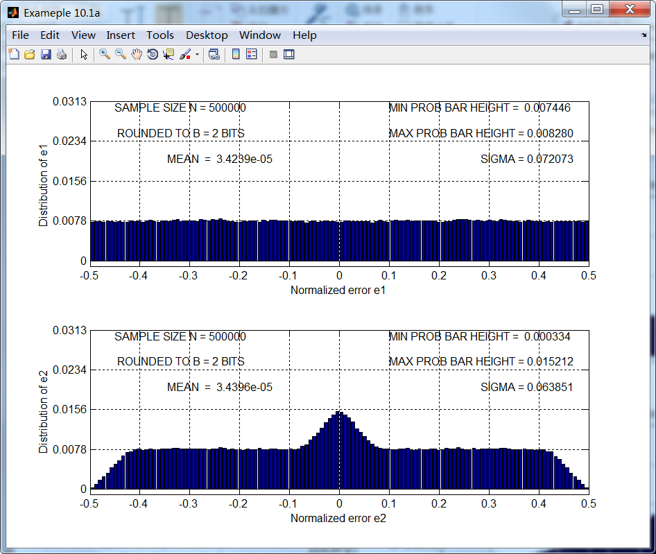
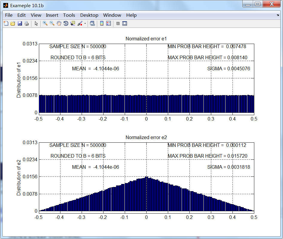
      B=2的结果如第1张图所示，很明显，即使误差看起来均匀分布，但误差采样序列不是独立的。对应B=6的
结果如第2张图所示，当B≥6时，结果满足误差模型假设条件。