如何入门Pytorch之一：Pytorch基本知识介绍

前言

       PyTorch和Tensorflow是目前最为火热的两大深度学习框架，Tensorflow主要用户群在于工业界，而PyTorch主要用户分布在学术界。目前视觉三大顶会的论文大多都是基于PyTorch，如何快速入门PyTorch成了当务之急。

正文

      本着循序渐进的原则，我会依次从易到难的内容进行介绍，并采用定期更新的方式来补充该文。

一、安装PyTorch 

      参考链接：https://blog.csdn.net/miao0967020148/article/details/80394270

      安装PyTorch前需要先安装Anaconda，然后使用如下命令

      conda install pytorch torchvision cuda80 -c soumith  { for cuda8.0  }

      conda install pytorch torchvision -c soumith         { for cuda7.5  }

      pip3 install -i https://pypi.tuna.tsinghua.edu.cn/simple torch==1.3.1  (sudo apt install python3-pip)

      pip3 install -i https://pypi.tuna.tsinghua.edu.cn/simple torchvision==0.4.2(同时会装上Torch1.3.1)

二、搭建第一个神经网络

一个简单的神经网络包含这些内容（数据准备，可调节参数，网络模型，损失函数，优化器）

1）数据准备

     x,y=get_data()

2) 可调节参数

    w,b=get_weight()

3) 网络模型

    y_pred = simple_network(x)         {y = wx+b }

4)损失函数

    loss = loss_fn(y,y_pred)     

5)优化器

   optimize(learning_rate)   

完整的神经网络如下：

x,y = get_data() # x - represents training data,y - represents target variables
w,b = get_weights() # w,b - Learnable parameters
for i in range(500):
    y_pred = simple_network(x) # function which computes wx + b
    loss = loss_fn(y,y_pred) # calculates sum of the squared differences of y and y_pred
if i % 50 == 0:
    print(loss)
    optimize(learning_rate) # Adjust w,b to minimize the loss

三、数据准备

     在PyTorch中，有两种类型的数据：1、张量；2.变量。其中Tensors类似于Numpy，就象Python中的Arrays，可以动态地修改大小。比如：一张正常的图像，可以用三维张量来表达，我们可以动态地放大到5维的张量。接下来逐一介绍各个维度的张量：

3.1张量

1）标量Scalar（0维张量）

x = torch.rand(10)
x.size()
Output - torch.Size([10])

2）向量Vector（1维张量）

temp = torch.FloatTensor([23,24,24.5,26,27.2,23.0])
temp.size()
Output - torch.Size([6])

3）矩阵Matrix（2维张量）

from sklearn.datasets import load_boston
boston=load_boston()
boston_tensor = torch.from_numpy(boston.data)
boston_tensor.size()
Output: torch.Size([506, 13])
boston_tensor[:2]
Output:
Columns 0 to 7
0.0063 18.0000 2.3100 0.0000 0.5380 6.5750 65.2000 4.0900
0.0273 0.0000 7.0700 0.0000 0.4690 6.4210 78.9000 4.9671
Columns 8 to 12
1.0000 296.0000 15.3000 396.9000 4.9800
2.0000 242.0000 17.8000 396.9000 9.1400
[torch.DoubleTensor of size 2x13]

4）3维张量Tensor

一张图片在内存空间中就是3维的。

from PIL import Image
import matplotlib.pyplot as plt
# Read a panda image from disk using a library called PIL and convert it to numpy array
panda = np.array(Image.open('panda.jpg').resize((224,224)))
panda_tensor = torch.from_numpy(panda)
panda_tensor.size()
Output - torch.Size([224, 224, 3])
#Display panda
plt.imshow(panda)

5）4维张量Tensor

一张图片为3维的Tensor，4维的张量就是多张图片的组合。使用GPU，我们可以一次性导入多张图片用来训练，导入的图片张数取决于GPU内存大小，一般情况下，批量导入的大小为16，32，64。

#Read cat images from disk
cats = glob(data_path+'*.jpg')
#Convert images into numpy arrays
cat_imgs = np.array([np.array(Image.open(cat).resize((224,224))) for cat in cats[:64]])
cat_imgs = cat_imgs.reshape(-1,224,224,3)
cat_tensors = torch.from_numpy(cat_imgs)
cat_tensors.size()
Output - torch.Size([64, 224, 224, 3])

6）5维张量Tensor

视频文件一般为5维的张量，在处理视频时，我们通常是把视频分解成一帧帧的图片，可以存储为[1,f,w,h,3]。而同时处理多个视频时，就是5维张量。

7)  切片张量Slicing Tensor

sales = torch.FloatTensor([1000.0,323.2,333.4,444.5,1000.0,323.2,333.4,444.5])
sales[:5]
1000.0000
323.2000
333.4000
444.5000
1000.0000
[torch.FloatTensor of size 5]
sales[:-5]
1000.0000
323.2000
333.4000
[torch.FloatTensor of size 3]

显示单维图片：

plt.imshow(panda_tensor[:,:,0].numpy())
#0 represents the first channel of RGB

显示裁剪图片：

plt.imshow(panda_tensor[25:175,60:130,0].numpy())

生成一个全为1矩阵：

#torch.eye(shape) produces an diagonal matrix with 1 as it diagonal #elements.
sales = torch.eye(3,3)
sales[0,1]

8）GPU中张量Tensor

（1） TensorCPU操作

#Various ways you can perform tensor addition
a = torch.rand(2,2)
b = torch.rand(2,2)
c = a + b
d = torch.add(a,b)
#For in-place addition
a.add_(5)
#Multiplication of different tensors
a*b
a.mul(b)
#For in-place multiplication
a.mul_(b)

（2） TensorGPU操作

a = torch.rand(10000,10000)
b = torch.rand(10000,10000)
a.matmul(b)
Time taken: 3.23 s
#Move the tensors to GPU
a = a.cuda()
b = b.cuda()
a.matmul(b)
Time taken: 11.2 μs

3.2 变量

深度学习算法经常是以计算图的形式出现，如下图：

 一个梯度类描述如下：

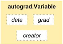
 梯度是关于y=wx+b中(w,b)的损失函数的改变率。

import torch
from torch.autograd import Variable

x =torch.autograd.Variable(torch.ones(2,2),requires_grad=True) 
y = x.mean() 
y.backward() #用于计算梯度 
x.grad Variable 
containing: 0.2500 0.2500 0.2500 0.2500 [torch.FloatTensor of size 2x2] 
x.grad_fn 
Output - None 
x.data 1 1 1 1 [torch.FloatTensor of size 2x2] 
y.grad_fn <torch.autograd.function.MeanBackward at 0x7f6ee5cfc4f8>

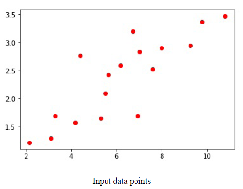
3.3 为自己搭建的模型准备数据

def get_data():
train_X = np.asarray([3.3,4.4,5.5,6.71,6.93,4.168,9.779,6.182,7.59,2.167,
7.042,10.791,5.313,7.997,5.654,9.27,3.1])
train_Y = np.asarray([1.7,2.76,2.09,3.19,1.694,1.573,3.366,2.596,2.53,1.221,
2.827,3.465,1.65,2.904,2.42,2.94,1.3])
dtype = torch.FloatTensor
X = Variable(torch.from_numpy(train_X).type(dtype),requires_grad=False).view(17,1)
y = Variable(torch.from_numpy(train_Y).type(dtype),requires_grad=False)
return X,y

3.4 搭建可学习参数

def get_weights():
w = Variable(torch.randn(1),requires_grad = True)
b = Variable(torch.randn(1),requires_grad = True)
return w,b

3.5 神经网络模型

    一旦我们定义了输入与输出，接下来要做的就是搭建神经网络模型。比如：y=wx+b,w和b就是可学习参数。

下图是一个拟合好的模型：

 

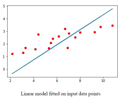
 图中蓝色线为拟合好的线。

模型完成

def simple_network(x):
y_pred = torch.matmul(x,w)+b
return y_pred

f = nn.Linear(17,1) # Much simpler.

3.6 损失函数

基于本文所探讨的回归问题，我们采用了均方差SSE的损失函数。torch.nn 有损失函数MSE和交叉熵损失。

def loss_fn(y,y_pred):
    loss = (y_pred-y).pow(2).sum()
    for param in [w,b]:
        if not param.grad is None: param.grad.data.zero_()  #由于梯度需要计算多次，这里要定期的对梯度值进行清零。
        loss.backward()
    return loss.data[0]

3.7 优化神经网络

损失函数计算完loss后，要对梯度值迭代计算更新，把梯度值和学习率代入进来，产生新的w，b。

def optimize(learning_rate):
w.data -= learning_rate * w.grad.data
b.data -= learning_rate * b.grad.data

不同的优化器如：Adam，RMSProp，SGD可以在torch.optim包中找到，可以使用这些优化器来减小损失从而提高精度。

3.8 加载数据

有两种重要类：Dataset和DataLoader

3.8.1 Dataset

原子类：

from torch.utils.data import Dataset
class DogsAndCatsDataset(Dataset):
def __init__(self,):
    pass
def __len__(self):
    pass
def __getitem__(self,idx):
    pass

添加了部分内容：

class DogsAndCatsDataset(Dataset):
def __init__(self,root_dir,size=(224,224)):
    self.files = glob(root_dir)
    self.size = size
def __len__(self):
    return len(self.files)
def __getitem__(self,idx):
    img = np.asarray(Image.open(self.files[idx]).resize(self.size))
    label = self.files[idx].split('/')[-2]
    return img,label

for image,label in dogsdset:
#Apply your DL on the dataset.

3.8.2 DataLoader

dataloader = DataLoader(dogsdset,batch_size=32,num_workers=2)
for imgs , labels in dataloader:
#Apply your DL on the dataset.
pass

Pytorch有两个有用的包：torchvision,torchtext.

下一篇：

       如何入门Pytorch之二：如何搭建实用神经网络