3.0 A Neural Network Example
载入数据:
from tensorflow.examples.tutorials.mnist import input_data
mnist = input_data.read_data_sets("MNIST_data/", one_hot=True)
ont_hot:将数据集的标签转换为ont-hot编码, i.e. “4”:[0, 0, 0, 0, 1, 0, 0, 0, 0, 0]。
3.1 Setting things up
1.为训练数据创建placeholder变量
# Python optimisation variables
learning_rate = 0.5
epochs = 10
batch_size = 100

# declare the training data placeholders
# input x - for 28 x 28 pixels = 784
x = tf.placeholder(tf.float32, [None, 784])
# now declare the output data placeholder - 10 digits
y = tf.placeholder(tf.float32, [None, 10])
2.创建一个三层神经网络的weights和bias
# now declare the weights connecting the input to the hidden layer
W1 = tf.Variable(tf.random_normal([784, 300], stddev=0.03), name='W1')
b1 = tf.Variable(tf.random_normal([300]), name='b1')
# and the weights connecting the hidden layer to the output layer
W2 = tf.Variable(tf.random_normal([300, 10], stddev=0.03), name='W2')
b2 = tf.Variable(tf.random_normal([10]), name='b2')
hidden layer有300个神经元。
tf.random_normal([784, 300], stddev=0.03):使用平均值为0,标准差为0.03的随机正态分布初始化weights和bias变量。
3.创建hidden layer的输入和激活函数:
# calculate the output of the hidden layer
hidden_out = tf.add(tf.matmul(x, W1), b1)
hidden_out = tf.nn.relu(hidden_out)
tf.matmul:矩阵乘法
这两行代码与下面两个等式等价:
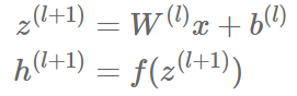
4.创建输出层:
# now calculate the hidden layer output - in this case, let's use a softmax activated
# output layer
y_ = tf.nn.softmax(tf.add(tf.matmul(hidden_out, W2), b2))
这里使用softmax激活函数。
5.引入一个loss function用于反向传播算法优化上述weight和bias。这里使用交叉熵误差
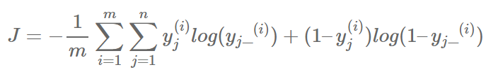
y_clipped = tf.clip_by_value(y_, 1e-10, 0.9999999)
cross_entropy = -tf.reduce_mean(tf.reduce_sum(y * tf.log(y_clipped) + (1 - y) * tf.log(1 - y_clipped), axis=1))
第一行:
将y_转换为剪辑版本(clipped version),取值位于1e-10,0.999999之间,是为了避免在训练时遇见log(0)而返回NaN并中止训练。
第二行:
tensor间的标量运算* / + -,
tensor*tensor:对两个tensor中的对应位置元素都进行运算。
tensor*scaler:对tensor中每个元素乘scaler。
tf.reduce_sum:按给定的坐标进行加和运算:
y * tf.log(y_clipped) + (1 - y) * tf.log(1 - y_clipped) 的运算结果是一个m*10的tensor。第一求和运算是对下标j求和,所以是对tensor的第2维进行求和,所以axis=1;得到结果是1*10的tensor。
tf.reduce_mean :对任何tensor求均值。
6.创建一个optimiser:
# add an optimiser
optimiser = tf.train.GradientDescentOptimizer(learning_rate=learning_rate).minimize(cross_entropy)
使用tensorflow提供的梯度下降优化器。
7.初始化所有变量和衡量准确度的运算。
# finally setup the initialisation operator
init_op = tf.global_variables_initializer()

# define an accuracy assessment operation
correct_prediction = tf.equal(tf.argmax(y, 1), tf.argmax(y_, 1))
accuracy = tf.reduce_mean(tf.cast(correct_prediction, tf.float32))
tf.equal:根据传入参数判断是否相等,返回True or False。
tf.argmax(tensor, axis):根据axis返回tensor中的最大值。返回的也是一个tensor。
correct_prediction:m*1的boolean tensor。
将其转换为float,然后计算平均值,就是准确率。
8.执行训练:
# start the session
with tf.Session() as sess:
   # initialise the variables
   sess.run(init_op)
   total_batch = int(len(mnist.train.labels) / batch_size)
   for epoch in range(epochs):
        avg_cost = 0
        for i in range(total_batch):
            batch_x, batch_y = mnist.train.next_batch(batch_size=batch_size)
             _, c = sess.run([optimiser, cross_entropy], feed_dict={x: batch_x, y: batch_y})
            avg_cost += c / total_batch
        print("Epoch:", (epoch + 1), "cost =", "{:.3f}".format(avg_cost))
   print(sess.run(accuracy, feed_dict={x: mnist.test.images, y: mnist.test.labels}))
使用mini-batch gradient descent。