Learning Efficient Convolutional Networks through Network Slimming
Zhuang Liu1∗ Jianguo Li2 Zhiqiang Shen3 Gao Huang4 Shoumeng Yan2 Changshui Zhang1
1CSAI, TNList, Tsinghua University 2Intel Labs China 3Fudan University 4Cornell University {liuzhuangthu, zhiqiangshen0214}@gmail.com, {jianguo.li, shoumeng.yan}@intel.com, gh349@cornell.edu, zcs@mail.tsinghua.edu.cn
Abstract
The deployment of deep convolutional neural networks (CNNs) in many Real-World applications is largely hindered by their high computational cost. In this paper, we propose a novel learning scheme for CNNs to simultaneously 1) reduce the model size; 2) decrease the run-time memory footprint; and 3) lower the number of computing operations, without compromising accuracy. This is achieved by enforcing channel-level sparsity in the network in a simple but effective way. Different from many existing approaches, the proposed method directly applies to modern CNN architectures, introduces minimum overhead to the training process, and requires no special software/hardware accelerators for the resulting models. We call our approach network slimming, which takes wide and large networks as input models, but during training insignificant channels are automatically identified and pruned afterwards, yielding thin and compact models with comparable accuracy. We empirically demonstrate the effectiveness of our approach with several state-of-the-art CNN models, including VGGNet, ResNet and DenseNet, on various image classification datasets. For VGGNet, a multi-pass version of network slimming gives a 20× reduction in model size and a 5× reduction in computing operations.
在许多实际应用中部署深度卷积神经网络(CNN)很大程度上受到其计算成本高的限制。在本文中,我们提出了一种新的CNNs学习方案,能同时1)减小模型大小; 2)减少运行时内存占用; 3)在不影响准确率的情况下降低计算操作的数量。这种学习方案是通过在网络中进行通道层次稀疏来实现,简单而有效。与许多现有方法不同,我们所提出的方法直接应用于现代CNN架构,引入训练过程的开销最小,并且所得模型不需要特殊软件/硬件加速器。我们将我们的方法称为网络瘦身(network slimming),此方法以大型网络作为输入模型,但在训练过程中,无关紧要的通道被自动识别和剪枝,从而产生精度相当但薄而紧凑(高效)的模型。在几个最先进的CNN模型(包括VGGNet,ResNet和DenseNet)上,我们使用各种图像分类数据集,凭经验证明了我们方法的有效性。对于VGGNet,网络瘦身后的多通道版本使模型大小减少20倍,计算操作减少5倍。
1. Introduction
In recent years, convolutional neural networks (CNNs) have become the dominant approach for a variety of computer vision tasks, e.g., image classification [22], object detection [8], semantic segmentation [26]. Large-scale datasets, high-end modern GPUs and new network architectures allow the development of unprecedented large CNN models. For instance, from AlexNet [22], VGGNet [31] and GoogleNet [34] to ResNets [14], the ImageNet Classification Challenge winner models have evolved from 8 layers to more than 100 layers.
近年来,卷积神经网络(CNN)已成为各种计算机视觉任务的主要方法,例如图像分类[22],物体检测[8],语义分割[26]。 大规模数据集,高端现代GPU和新的网络架构允许开发前所未有的大型CNN模型。 例如,从AlexNet [22],VGGNet [31]和GoogleNet [34]到ResNets [14],ImageNet分类挑战赛冠军模型已经从8层发展到100多层。
However, large CNNs, although with stronger representation power, are more resource-hungry. For instance, a 152-layer ResNet [14] has more than 60 million parameters and requires more than 20 Giga float-point-operations (FLOPs) when inferencing an image with resolution 224× 224. This is unlikely to be affordable on resource constrained platforms such as mobile devices, wearables or Internet of Things (IoT) devices.
然而,大型CNN虽然具有更强的代表(表现,提取特征,表征)能力,却也更耗费资源。 例如,一个152层的ResNet [14]具有超过6000万个参数,在推测(处理)分辨率为224×224的图像时需要超过20个Giga的浮点运算(FLOP)-即20G flop的运算量。这在资源受限的情况下不可能负担得起,如在移动设备,可穿戴设备或物联网(IoT)设备等平台上。
The deployment of CNNs in real world applications are mostly constrained by 1) Model size: CNNs’ strong representation power comes from their millions of trainable parameters. Those parameters, along with network structure information, need to be stored on disk and loaded into memory during inference time. As an example, storing a typical CNN trained on ImageNet consumes more than 300MB space, which is a big resource burden to embedded devices. 2) Run-time memory: During inference time, the intermediate activations/responses of CNNs could even take more memory space than storing the model parameters, even with batch size 1. This is not a problem for high-end GPUs, but unaffordable for many applications with low computational power. 3) Number of computing operations: The convolution operations are computationally intensive on high resolution images. A large CNN may take several minutes to process one single image on a mobile device, making it unrealistic to be adopted for real applications.
CNN在实际应用中的部署主要受以下因素的限制:1)模型大小:CNN的强大表现力来自其数百万可训练参数。这些参数以及网络结构信息需要存储在磁盘上并在推理期间加载到内存中。例如,存储一个ImageNet上训练的典型CNN会占用超过300MB的空间,这对嵌入式设备来说是一个很大的资源负担。 2)运行时内存(占用情况):在推理期间,即使批量大小为1,CNN的中间激活/响应占用的内存空间甚至可以比存储模型的参数更多.这对于高端GPU来说不是问题,但是对于许多计算能力低的应用而言是无法承受的。 3)计算操作的数量:在高分辨率图像的卷积操作上是计算密集的。大型CNN在移动设备上处理单个图像可能需要几分钟,这使得在实际应用中采用大型CNN是不现实的。
Many works have been proposed to compress large CNNs or directly learn more efficient CNN models for fast inference. These include low-rank approximation [7], network quantization [3, 12] and binarization [28, 6], weight pruning [12], dynamic inference [16], etc. However, most of these methods can only address one or two challenges mentioned above. Moreover, some of the techniques require specially designed software/hardware accelerators for execution speedup [28, 6, 12].
许多工作已经提出了压缩大型CNN或直接学习更有效的CNN模型以进行快速推理。 这些工作包括低秩逼近(这么翻译正确吗?)[7],网络量化[3,12]和网络二值化[28,6],权重剪枝[12],动态推理[16]等。但是,这些方法大多数只能解决一个或两个上面提到的挑战。 此外,一些技术需要专门设计的软件/硬件加速器来实行加速[28,6,12]。
Another direction to reduce the resource consumption of large CNNs is to sparse the network. Sparsity can be imposed on different level of structures [2, 37, 35, 29, 25], which yields considerable model-size compression and inference speedup. However, these approaches generally require special software/hardware accelerators to harvest the gain in memory or time savings, though it is easier than non-structured sparse weight matrix as in [12].
减少大型CNN资源消耗的另一个方向是稀疏化网络。 可以对不同级别的结构施加稀疏性[2,37,35,29,25],这产生了相当大的模型大小压缩和推理加速。 尽管它比[12]中的非结构化稀疏权重矩阵更容易,然而,这些方法通常需要特殊的软件/硬件加速器来获得内存增益或节省时间。
In this paper, we propose network slimming, a simple yet effective network training scheme, which addresses all the aforementioned challenges when deploying large CNNs under limited resources. Our approach imposes L1 regularization on the scaling factors in batch normalization (BN) layers, thus it is easy to implement without introducing any change to existing CNN architectures. Pushing the values of BN scaling factors towards zero with L1 regularization enables us to identify insignificant channels (or neurons), as each scaling factor corresponds to a specific convolutional channel (or a neuron in a fully-connected layer). This facilitates the channel-level pruning at the followed step. The additional regularization term rarely hurt the performance. In fact, in some cases it leads to higher generalization accuracy. Pruning unimportant channels may sometimes temporarily degrade the performance, but this effect can be compensated by the followed fine-tuning of the pruned network. After pruning, the resulting narrower network is much more compact in terms of model size, runtime memory, and computing operations compared to the initial wide network. The above process can be repeated for several times, yielding a multi-pass network slimming scheme which leads to even more compact network.
在本文中,我们提出了网络瘦身,这是一种简单而有效的网络训练方案,它解决了在有限资源的条件下应用大型CNN时所面临的所有挑战。我们的方法对批量归一化(BN)层中的缩放因子强加L1正则化,因此很容易实现,而不会对现有CNN架构进行任何更改。通过L1正则化将BN缩放因子的值逼近零使得我们能够识别不重要的通道(或神经元),因为每个缩放因子对应于特定的卷积通道(或完全连接的层中的神经元)。这有助于在随后的步骤中进行通道层次的修剪。额外的正则化术语很少会影响性能。实际上,在某些情况下,它会导致更高的泛化精度。修剪不重要的通道有时会暂时降低性能,但是这种影响可以通过修剪网络的后续调整来补偿。修剪后,与初始的大型网络相比,由此产生的轻量化网络在模型大小,运行时内存和计算操作方面更加紧凑。上述过程可以重复多次以产生多通道网络瘦身方案,这能产生更紧凑的网络。
Experiments on several benchmark datasets and different network architectures show that we can obtain CNN models with up to 20x mode-size compression and 5x reduction in computing operations of the original ones, while achieving the same or even higher accuracy. Moreover, our method achieves model compression and inference speedup with conventional hardware and deep learning software packages, since the resulting narrower model is free of any sparse storing format or computing operations.
在几个基准数据集和不同网络架构上的实验表明,我们获得的CNN模型,其大小压缩高达20倍,原始计算操作减少5倍,同时实现了相同甚至更高的精度。此外,我们的方法利用传统硬件和深度学习软件包实现模型压缩和推理加速,因此得到的轻量化模型不需要任何稀疏存储格式或特殊的计算操作。
2. Related Work
In this section, we discuss related work from five aspects. Low-rank Decomposition approximates weight matrix in neural networks with low-rank matrix using techniques like Singular Value Decomposition (SVD) [7]. This method works especially well on fully-connected layers, yielding ∼3x model-size compression however without notable speed acceleration, since computing operations in CNN mainly come from convolutional layers.
在本节中,我们将从五个方面讨论相关工作。用奇异值分解(SVD)等技术使具有较低秩的矩阵去逼近神经网络中的权重矩阵[7]。 这种方法在全连接的层上工作得特别好,产生~3倍模型大小的压缩,但没有明显的速度加速,因为CNN中的计算操作主要来自卷积层。
Weight Quantization. HashNet [3] proposes to quantize the network weights. Before training, network weights are hashed to different groups and within each group weight the value is shared. In this way only the shared weights and hash indices need to be stored, thus a large amount of storage space could be saved. [12] uses a improved quantization technique in a deep compression pipeline and achieves 35x to 49x compression rates on AlexNet and VGGNet. However, these techniques can neither save run-time memory nor inference time, since during inference shared weights need to be restored to their original positions.
权重量化。 HashNet [3]建议量化网络权重。 在训练之前,网络权重被散列到不同的组,并且在每个组内共享该权重值。 这样,只需要存储共享权重和哈希索引,从而可以节省大量的存储空间。 [12]在深度压缩流程中使用改进的量化技术,在AlexNet和VGGNet上实现35x到49x的压缩率。 但是,这些技术既不能节省运行时内存也不能节省推理时间,因为在推理期间,需要将共享权重恢复到其原始位置。
[28, 6] quantize real-valued weights into binary/ternary weights (weight values restricted to {−1,1} or {−1,0,1}). This yields a large amount of model-size saving, and significant speedup could also be obtained given bitwise operation libraries. However, this aggressive low-bit approximation method usually comes with a moderate accuracy loss.
[28,6]将实值权重量化为二进制/三进制权重(权重值限制为{-1,1}或{-1,0,1})。 这样可以节省大量的模型空间,并且在给定按位运算库的情况下也可以获得显着的加速。 然而,这种积极的(意思是压缩力度过大?)低位近似方法通常具有一定的精度损失。
Weight Pruning / Sparsifying. [12] proposes to prune the unimportant connections with small weights in trained neural networks. The resulting network’s weights are mostly zeros thus the storage space can be reduced by storing the model in a sparse format. However, these methods can only achieve speedup with dedicated sparse matrix operation libraries and/or hardware. The run-time memory saving is also very limited since most memory space is consumed by the activation maps (still dense) instead of the weights.
权重剪枝/稀疏。 [12]提出在训练好的神经网络中修剪不重要的小权重连接。 由此产生的网络权重大多为零,可以通过以稀疏格式存储模型来减少存储空间。 但是,这些方法只能通过专用的稀疏矩阵运算库和/或硬件实现加速。 运行时内存节省也非常有限,因为大多数内存空间被激活映射(仍然密集)而不是权重消耗。
In [12], there is no guidance for sparsity during training. [32] overcomes this limitation by explicitly imposing sparse constraint over each weight with additional gate variables, and achieve high compression rates by pruning connections with zero gate values. This method achieves better com pression rate than [12], but suffers from the same drawback.
在[12]中,没有关于训练期间如何稀疏的指导。 [32]通过使用额外的门变量明确地对每个权重施加稀疏约束来克服此限制,并通过修剪具有零门值的连接来实现高压缩率。 该方法实现了比[12]更好的压缩率,但也存在同样的缺点。
Structured Pruning / Sparsifying. Recently, [23] proposes to prune channels with small incoming weights in trained CNNs, and then fine-tune the network to regain accuracy. [2] introduces sparsity by random deactivating input-output channel-wise connections in convolutional layers before training, which also yields smaller networks with moderate accuracy loss. Compared with these works, we explicitly impose channel-wise sparsity in the optimization objective during training, leading to smoother channel pruning process and little accuracy loss.
结构化修剪/稀疏化。 最近,[23]提出在训练好的CNN中修剪具有较小输入权重的信道,然后对网络进行微调以恢复准确性。 [2]通过在训练之前在卷积层中随机停用输入 - 输出信道连接的方式来引入稀疏性,这能产生具有中等精度损失的较小网络。 与这些工作相比,我们在训练期间明确地在优化目标中强加了通道方式稀疏性,导致更平滑的通道修剪过程和很少的准确性损失。
[37] imposes neuron-level sparsity during training thus some neurons could be pruned to obtain compact networks. [35] proposes a Structured Sparsity Learning (SSL) method to sparsify different level of structures (e.g. filters, channels or layers) in CNNs. Both methods utilize group sparsity regualarization during training to obtain structured sparsity. Instead of resorting to group sparsity on convolutional weights, our approach imposes simple L1 sparsity on channel-wise scaling factors, thus the optimization objective is much simpler.
[37]在训练期间强加神经元水平的稀疏性,因此可以修剪一些神经元以获得紧凑的网络。 [35]提出了一种结构化稀疏度学习(SSL)方法,用于稀疏CNN中不同级别的结构(例如滤波器,信道或层)。 两种方法都在训练期间利用群组稀疏性规则化来获得结构化稀疏性。 我们的方法不是在卷积权重上采用群稀疏度,而是在通道方面的缩放因子上强加简单的L1稀疏性,因此优化目标要简单得多。
Since these methods prune or sparsify part of the network structures (e.g., neurons, channels) instead of individual weights, they usually require less specialized libraries (e.g. for sparse computing operation) to achieve inference speedup and run-time memory saving. Our network slimming also falls into this category, with absolutely no special libraries needed to obtain the benefits.
由于这些方法修剪或稀疏网络结构的一部分(例如,神经元,信道)而不是单独的权重,它们通常需要较少的专用库(例如,用于稀疏计算操作)以实现推理加速和运行时存储器节省。 我们的网络瘦身也属于这一类,完全不需要特殊的库来获得增益。
Neural Architecture Learning. While state-of-the-art CNNs are typically designed by experts [22, 31, 14], there are also some explorations on automatically learning network architectures. [20] introduces sub-modular/supermodular optimization for network architecture search with a given resource budget. Some recent works [38, 1] propose to learn neural architecture automatically with reinforcement learning. The searching space of these methods are extremely large, thus one needs to train hundreds of models to distinguish good from bad ones. Network slimming can also be treated as an approach for architecture learning, despite the choices are limited to the width of each layer. However, in contrast to the aforementioned methods, network slimming learns network architecture through only a single training process, which is in line with our goal of efficiency.
神经结构学习。 虽然最先进的CNN通常由专家[22,31,14]设计,但也有一些关于自动学习网络架构的探索。 [20]引入了用于给定资源预算的网络架构搜索的子模块/超模块优化。 最近的一些工作[38,1]提出通过强化学习自动学习神经结构。 这些方法的搜索空间非常大,因此需要训练数百个模型来区分好与坏。 网络瘦身也可以被视为架构学习的一种方法,尽管选择仅限于每层的宽度。 然而,与上述方法相比,网络瘦身仅通过一个训练过程来学习网络架构,这符合我们的效率目标。
3. Network slimming
We aim to provide a simple scheme to achieve channel-level sparsity in deep CNNs. In this section, we first discuss the advantages and challenges of channel-level sparsity, and introduce how we leverage the scaling layers in batch normalization to effectively identify and prune unimportant channels in the network.
我们的目标是提供一个简单的方案来实现深度CNN中的信道层次的稀疏。 在本节中,我们首先讨论了信道层次稀疏的优势和挑战,并介绍了如何利用批量规范化中的扩展层(缩放因子)来有效地识别和修剪网络中不重要的信道。
Advantages of Channel-level Sparsity. As discussed in prior works [35, 23, 11], sparsity can be realized at different levels, e.g., weight-level, kernel-level, channel-level or layer-level. Fine-grained level (e.g., weight-level) sparsity gives the highest flexibility and generality leads to higher compression rate, but it usually requires special software or hardware accelerators to do fast inference on the sparse model [11]. On the contrary, the coarsest layer-level sparsity does not require special packages to harvest the inference speedup, while it is less flexible as some whole layers need to be pruned. In fact, removing layers is only effective when the depth is sufficiently large, e.g., more than 50 layers [35, 18]. In comparison, channel-level sparsity provides a nice tradeoff between flexibility and ease of implementation. It can be applied to any typical CNNs or fully connected networks (treat each neuron as a channel), and the resulting network is essentially a “thinned” version of the unpruned network, which can be efficiently inferenced on conventional CNN platforms.
通道层次稀疏性的优势。如在先前的工作[35,23,11]中所讨论的,稀疏性可以在不同的层次实现,例如,权重级,内核级,通道级或层级。细粒度级别(例如,权重级别)稀疏性提供最高的灵活性和通用性导致更高的压缩率,但它通常需要特殊的软件或硬件加速器来对稀疏模型进行快速推理[11]。相反,粗糙层级稀疏性不需要特殊的包来获得推理加速,而它不太灵活,因为需要修剪一些整个层。实际上,去除整层仅在模型深度足够大时才有效,例如,超过50层[35,18]。相比之下,通道层次稀疏性提供了灵活性和易于实现之间的良好折衷。它可以应用于任何典型的CNN或全连接的网络(将每个神经元视为信道),并且所得到的网络本质上是未修整网络的“稀疏”版本,其可以在传统CNN平台上被有效地推断。
Challenges. Achieving channel-level sparsity requires pruning all the incoming and outgoing connections associated with a channel. This renders the method of directly pruning weights on a pre-trained model ineffective, as it is unlikely that all the weights at the input or output end of a channel happen to have near zero values. As reported in [23], pruning channels on pre-trained ResNets can only lead to a reduction of∼10% in the number of parameters without suffering from accuracy loss. [35] addresses this problem by enforcing sparsity regularization into the training objective. Specifically, they adopt group LASSO to push all the filter weights corresponds to the same channel towards zero simultaneously during training. However, this approach requires computing the gradients of the additional regularization term with respect to all the filter weights, which is nontrivial. We introduce a simple idea to address the above challenges, and the details are presented below.
挑战。 实现通道层次稀疏性需要修剪与通道关联的所有传入和传出连接,这使得在预训练模型上直接修剪权重的方法无效,因为通道的输入或输出端处的所有权重不可能恰好具有接近零的值。 如[23]所述,预训练的ResNets上的通道修剪只能减少参数数量的~10%才不会导致精度损失。 [35]通过将稀疏正规化强制纳入训练目标来解决这个问题。 具体而言,他们采用组LASSO在训练期间将所有对应于同一通道的滤波器权重同时逼近零。 然而,这种方法需要相对于所有滤波器权重来计算附加正则化项的梯度,这是非常重要的。 我们引入一个简单的想法来解决上述挑战,详情如下。
Scaling Factors and Sparsity-induced Penalty. Our idea is introducing a scaling factor γ for each channel, which is multiplied to the output of that channel. Then we jointly train the network weights and these scaling factors, with sparsity regularization imposed on the latter. Finally we prune those channels with small factors, and fine-tune the pruned network. Specifically, the training objective of our approach is given by
缩放因素和稀疏性惩罚。 我们的想法是为每个通道引入一个比例因子γ,它乘以该通道的输出。 然后我们联合训练网络权重和这些比例因子,并对后者施加稀疏正则化。 最后,我们修剪这些小因子通道,并调整修剪后的网络。 具体而言,我们的方法的训练目标是:
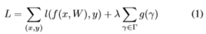
where (x, y) denote the train input and target, W denotes the trainable weights, the first sum-term corresponds to the normal training loss of a CNN, g(·) is a sparsity-induced penalty on the scaling factors, and λ balances the two terms. In our experiment, we choose g(s)=|s|, which is known as L1-norm and widely used to achieve sparsity. Subgradient descent is adopted as the optimization method for the nonsmooth L1 penalty term. An alternative option is to replace the L1 penalty with the smooth-L1 penalty [30] to avoid using sub-gradient at non-smooth point.
其中(x,y)表示训练输入和目标,W表示可训练的权重,第一个和项对应于CNN的正常训练损失,g(·)是比例因子的稀疏性引起的惩罚,以及 λ平衡这两个损失。 在我们的实验中,我们选择g(s)= | s |,它被称为L1范数并广泛用于实现稀疏性。 采用次梯度下降作为非光滑L1惩罚项的优化方法。 另一种选择是将L1惩罚替换为平滑L1惩罚[30],以避免在非平滑点使用子梯度。
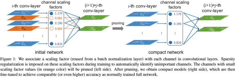
As pruning a channel essentially corresponds to removing all the incoming and outgoing connections of that channel, we can directly obtain a narrow network (see Figure 1) without resorting to any special sparse computation packages. The scaling factors act as the agents for channel selection. As they are jointly optimized with the network weights, the network can automatically identity insignificant channels, which can be safely removed without greatly affecting the generalization performance.
修剪一个通道基本上对应于删除该通道的所有传入和传出连接,我们可以直接获得一个轻量化的网络(见图1),而不需要使用任何特殊的稀疏计算包。 缩放因子充当频道选择的代理。 由于它们与网络权重共同优化,因此网络可以自动识别无关紧要的通道,这些通道可以安全地移除而不会极大地影响泛化性能。
Leveraging the Scaling Factors in BN Layers. Batch normalization [19] has been adopted by most modern CNNs as a standard approach to achieve fast convergence and better generalization performance. The way BN normalizes the activations motivates us to design a simple and efficient method to incorporates the channel-wise scaling factors. Particularly, BN layer normalizes the internal activations using mini-batch statistics. Let zin and zout be the input and output of a BN layer, B denotes the current minibatch, BN layer performs the following transformation:
利用BN图层中的缩放因子。 批量归一化[19]已被大多数现代CNN采用作为实现快速收敛和更好的泛化性能的标准方法。 BN规范化激活的方式促使我们设计一种简单有效的方法来合并通道方式的缩放因子。 特别地,BN层使用小批量统计来标准化内部激活。 令zin和zout为BN层的输入和输出,B表示当前的小批量,BN层执行以下转换:
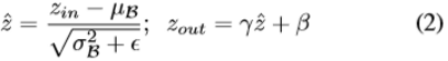
where µB and σB are the mean and standard deviation values of input activations over B, γ and β are trainable affine transformation parameters (scale and shift) which provides the possibility of linearly transforming normalized activations back to any scales.
其中μB和σB是B上输入激活的平均值和标准偏差值,γ和β是可以通过训练变换的参数(比例和偏移),这提供了将归一化激活线性转换到任何尺度的可能性。
It is common practice to insert a BN layer after a convolutional layer, with channel-wise scaling/shifting parameters. Therefore, we can directly leverage the γ parameters in BN layers as the scaling factors we need for network slimming. It has the great advantage of introducing no overhead to the network. In fact, this is perhaps also the most effective way we can learn meaningful scaling factors for channel pruning. 1), if we add scaling layers to a CNN without BN layer, the value of the scaling factors are not meaningful for evaluating the importance of a channel, because both convolution layers and scaling layers are linear transformations. One can obtain the same results by decreasing the scaling factor values while amplifying the weights in the convolution layers. 2), if we insert a scaling layer before a BN layer, the scaling effect of the scaling layer will be completely canceled by the normalization process in BN. 3), if we insert scaling layer after BN layer, there are two consecutive scaling factors for each channel.
通常的做法是在卷积层之后插入BN层,保留通道缩放/移位参数。因此,我们可以直接利用BN层中的γ参数作为网络瘦身所需的比例因子。它具有不向网络引入任何开销的巨大优势。事实上,这也许是我们学习有用的通道修剪缩放因子的最有效方法。 1),如果我们将缩放层添加到没有BN层的CNN,则缩放因子的值对于评估通道的重要性没有意义,因为卷积层和缩放层都是线性变换。通过放大卷积层中的权重的同时减小缩放因子值,可以获得相同的结果。 2),如果我们在BN层之前插入缩放层,缩放层的缩放效果将被BN中的归一化处理完全取消。 3),如果我们在BN层之后插入缩放层,则每个通道有两个连续的缩放因子。
Channel Pruning and Fine-tuning. After training under channel-level sparsity-induced regularization, we obtain a model in which many scaling factors are near zero (see Figure 1). Then we can prune channels with near-zero scaling factors, by removing all their incoming and outgoing connections and corresponding weights. We prune channels with a global threshold across all layers, which is defined as a certain percentile of all the scaling factor values. For instance, we prune 70% channels with lower scaling factors by choosing the percentile threshold as 70%. By doing so, we obtain a more compact network with less parameters and run-time memory, as well as less computing operations.
通道剪枝和微调。 在通道层次稀疏诱导正则化训练之后,我们获得了一个模型,其中许多比例因子接近于零(见图1)。 然后我们可以通过删除所有传入和传出连接以及相应的权重来修剪具有接近零比例因子的通道。 我们使用全局阈值在所有层上修剪通道,其被定义为所有比例因子值的特定百分位数。 例如,我们通过选择百分比阈值为70%来修剪具有较低缩放因子的70%通道。 通过这样做,我们获得了一个更紧凑的网络,具有更少的参数和运行时内存,以及更少的计算操作。
Pruning may temporarily lead to some accuracy loss, when the pruning ratio is high. But this can be largely compensated by the followed fine-tuning process on the pruned network. In our experiments, the fine-tuned narrow network can even achieve higher accuracy than the original unpruned network in many cases.
当修剪比例高时,修剪可能暂时导致一些精确度损失。 但是,这可以通过修剪网络上的后续微调过程得到很大程度的补偿。 在我们的实验中,在许多情况下,微调的轻量化网络甚至可以实现比原始未修网络更高的精度。
Multi-pass Scheme. We can also extend the proposed method from single-pass learning scheme (training with sparsity regularization, pruning, and fine-tuning) to a multi-pass scheme. Specifically, a network slimming procedure results in a narrow network, on which we could again apply the whole training procedure to learn an even more compact model. This is illustrated by the dotted-line in Figure 2. Experimental results show that this multi-pass scheme can lead to even better results in terms of compression rate.
多通道方案。 我们还可以将所提出的方法从单程学习方案(具有稀疏正则化,修剪和微调的训练)扩展到多程方案。 具体而言,网络瘦身过程导致网络狭窄,我们可以再次应用整个训练程序来学习更紧凑的模型。 这由图2中的虚线说明。实验结果表明,这种多次通过方案可以在压缩率方面产生更好的结果。

Handling Cross Layer Connections and Pre-activation Structure. The network slimming process introduced above can be directly applied to most plain CNN architectures such as AlexNet [22] and VGGNet [31]. While some adaptations are required when it is applied to modern networks with cross layer connections and the pre-activation design such as ResNet [15] and DenseNet [17]. For these networks, the output of a layer may be treated as the input of multiple subsequent layers, in which a BN layer is placed before the convolutional layer. In this case, the sparsity is achieved at the incoming end of a layer, i.e., the layer selectively uses a subset of channels it received. To harvest the parameter and computation savings at test time, we need to place a channel selection layer to mask out insignificant channels we have identified.
处理跨层连接和预激活结构。 上面介绍的网络瘦身过程可以直接应用于大多数简单的CNN架构,如AlexNet [22]和VGGNet [31]。 当它应用于具有跨层连接的现代网络和预激活设计(如ResNet [15]和DenseNet [17])时,需要进行一些调整。 对于这些网络,层的输出可以被视为多个后续层的输入,其中BN层被放置在卷积层之前。 在这种情况下,在层的输入端实现稀疏性,即,该层选择性地使用它接收的通道子集。 为了在测试时获得参数和计算节省,我们需要设置一个通道选择层来屏蔽我们识别出的无关紧要的通道。
4. Experiments
We empirically demonstrate the effectiveness of network slimming on several benchmark datasets. We implement our method based on the publicly available Torch [5] implementation for ResNets by [10]. The code is available at https://github.com/liuzhuang13/slimming
我们经验性地证明了网络瘦身对几个基准数据集的有效性。 我们基于[10]的ResNets的公开可用的Torch 版本[5]实现来验证我们的方法。 该代码可在https://github.com/liuzhuang13/slimming获得
4.1. Datasets
CIFAR. The two CIFAR datasets [21] consist of natural images with resolution 32×32. CIFAR-10 is drawn from 10 and CIFAR-100 from 100 classes. The train and test sets contain 50,000 and 10,000 images respectively. On CIFAR10, a validation set of 5,000 images is split from the training set for the search of λ (in Equation 1) on each model. We report the final test errors after training or fine-tuning on all training images. A standard data augmentation scheme (shifting/mirroring) [14, 18, 24] is adopted. The input data is normalized using channel means and standard deviations. We also compare our method with [23] on CIFAR datasets.
CIFAR。 两个CIFAR数据集[21]由分辨率为32×32的自然图像组成。 CIFAR-10有10个类,CIFAR-100有100个类。 训练和测试集分别包含50,000和10,000个图像。 在CIFAR10上,从训练集中分离出5,000个图像的验证集,用于在每个模型上搜索λ(在等式1中)。 我们在训练或微调所有训练图像后报告最终的测试错误。 采用标准数据增强方案(移位/镜像)[14,18,24]。 使用通道平均值和标准偏差对输入数据进行标准化。 我们还将我们的方法与[23]在CIFAR数据集上进行了比较。
SVHN. The Street View House Number (SVHN) dataset [27] consists of 32x32 colored digit images. Following common practice [9, 18, 24] we use all the 604,388 training images, from which we split a validation set of 6,000 images for model selection during training. The test set contains 26,032 images. During training, we select the model with the lowest validation error as the model to be pruned (or the baseline model). We also report the test errors of the models with lowest validation errors during fine-tuning.
SVHN。 街景房号(SVHN)数据集[27]由32x32彩色数字图像组成。 按照惯例[9,18,24],我们使用了所有604,388个训练图像,我们在训练期间从中分割出6,000个图像的验证集,用于模型选择。 测试集包含26,032个图像。 在训练期间,我们选择具有最低验证误差的模型作为要修剪的模型(或基线模型)。 我们还报告了模型的测试错误,在调整期间具有最低的验证错误。
ImageNet. The ImageNet dataset contains 1.2 million training images and 50,000 validation images of 1000 classes. We adopt the data augmentation scheme as in [10]. We report the single-center-crop validation error of the final model.
ImageNet。 ImageNet数据集包含120万个训练图像和50,000个验证图像,总共有1000个类。 我们采用[10]中的数据增强方案。 我们报告了最终模型的单中心作物验证错误。
MNIST. MNIST is a handwritten digit dataset containing 60,000 training images and 10,000 test images. To test the effectiveness of our method on a fully-connected network (treating each neuron as a channel with 1×1 spatial size), we compare our method with [35] on this dataset.
MNIST。 MNIST是一个手写的数字数据集,包含60,000个训练图像和10,000个测试图像。 为了测试我们的方法在完全连接的网络上的有效性(将每个神经元视为1×1空间大小的通道),我们将该方法与[35]在该数据集上进行比较
4.2. Network Models
On CIFAR and SVHN dataset, we evaluate our method on three popular network architectures: VGGNet[31], ResNet [14] and DenseNet [17]. The VGGNet is originally designed for ImageNet classification. For our experiment a variation of the original VGGNet for CIFAR dataset is taken from [36]. For ResNet, a 164-layer pre-activation ResNet with bottleneck structure (ResNet-164) [15] is used. For DenseNet, we use a 40-layer DenseNet with growth rate 12 (DenseNet-40).
在CIFAR和SVHN数据集上,我们在三种流行的网络架构上评估我们的方法:VGGNet [31],ResNet [14]和DenseNet [17]。 VGGNet最初是为ImageNet分类而设计的。 对于我们的实验,原始VGGNet的变体取自[36] 在CIFAR数据集的结果。 对于ResNet,使用具有瓶颈结构的164层预激活ResNet(ResNet-164)[15]。 对于DenseNet,我们使用40层DenseNet,增长率为12(DenseNet-40)。
On ImageNet dataset, we adopt the 11-layer (8-conv + 3 FC) “VGG-A” network [31] model with batch normalization from [4]. We remove the dropout layers since we use relatively heavy data augmentation. To prune the neurons in fully-connected layers, we treat them as convolutional channels with 1×1 spatial size.
在ImageNet数据集中,我们采用11层(8-conv + 3 FC)“VGG-A”网络[31]模型,并从[4]中进行批量归一化。 我们删除了dropout层,因为我们使用很多的数据扩充。 为了修剪完全连接层中的神经元,我们将它们视为具有1×1空间大小的卷积通道。
On MNIST dataset, we evaluate our method on the same 3-layer fully-connected network as in [35].
在MNIST数据集上,我们在与[35]中相同的3层全连接网络上评估我们的方法。
4.3. Training, Pruning and Fine-tuning
Normal Training. We train all the networks normally from scratch as baselines. All the networks are trained using SGD. On CIFAR and SVHN datasets we train using minibatch size 64 for 160 and 20 epochs, respectively. The initial learning rate is set to 0.1, and is divided by 10 at 50% and 75% of the total number of training epochs. On ImageNet and MNIST datasets, we train our models for 60 and 30 epochs respectively, with a batch size of 256, and an initial learning rate of 0.1 which is divided by 10 after 1/3 and 2/3 fraction of training epochs. We use a weight decay of 10−4 and a Nesterov momentum [33] of 0.9 without dampening. The weight initialization introduced by [13] is adopted. Our optimization settings closely follow the original implementation at [10]. In all our experiments, we initialize all channel scaling factors to be 0.5, since this gives higher accuracy for the baseline models compared with default setting (all initialized to be 1) from [10].
正常训练。 我们通常从头开始训练所有网络作为基线。 所有网络都使用SGD进行训练。 在CIFAR和SVHN数据集上,我们分别使用尺寸为64的小批量训练160和20个epochs。 初始学习率设置为0.1,并且在训练epoch总数的50%和75%处除以10。 在ImageNet和MNIST数据集上,我们分别训练60和30个epochs的模型,批量大小为256,初始学习率为0.1,在1/3和2/3的训练epoch之后除以10。 我们使用10-4的重量衰减和0.9的Nesterov动量[33],不使用权重衰减(对么?)。 采用[13]引入的权重初始化。 我们的优化设置参考[10]原始实现。 在我们的所有实验中,我们将所有通道缩放因子初始化为0.5,因为与[10]中的默认设置(全部初始化为1)相比,这为基线模型提供了更高的准确性。
Training with Sparsity. For CIFAR and SVHN datasets, when training with channel sparse regularization, the hyper parameter λ, which controls the tradeoff between empirical loss and sparsity, is determined by a grid search over 10−3, 10−4, 10−5 on CIFAR-10 validation set. For VGGNet we choose λ=10−4 and for ResNet and DenseNet λ=10−5. For VGG-A on ImageNet, we set λ=10−5. All other settings are kept the same as in normal training.
稀疏训练。 对于CIFAR和SVHN数据集,当使用通道稀疏正则化训练时,控制经验损失和稀疏度之间权衡的超参数λ由CIFAR-10上的10-3,10-4,10-5的网格搜索确定。 验证集。 对于VGGNet,我们选择λ= 10-4,对于ResNet和DenseNet,λ= 10-5。 对于ImageNet上的VGG-A,我们设置λ= 10-5。 所有其他设置保持与正常训练相同。
Pruning. When we prune the channels of models trained with sparsity, a pruning threshold on the scaling factors needs to be determined. Unlike in [23] where different layers are pruned by different ratios, we use a global pruning threshold for simplicity. The pruning threshold is determined by a percentile among all scaling factors , e.g., 40% or 60% channels are pruned. The pruning process is implemented by building a new narrower model and copying the corresponding weights from the model trained with sparsity.
修剪。 当我们修剪用稀疏性训练的模型的通道时,需要确定缩放因子的修剪阈值。 与[23]不同,不同的层以不同的比例进行修剪,为简单起见,我们使用全局修剪阈值。 修剪阈值由所有缩放因子中的百分位数确定,例如,修剪40%或60%的通道。 修剪过程是通过构建一个新的较窄的模型并从稀疏训练的模型中复制相应的权重来实现的。
Fine-tuning. After the pruning we obtain a narrower and more compact model, which is then fine-tuned. On CIFAR, SVHN and MNIST datasets, the fine-tuning uses the same optimization setting as in training. For ImageNet dataset, due to time constraint, we fine-tune the pruned VGG-A with a learning rate of 10−3 for only 5 epochs.
微调。 在修剪之后,我们获得了一个更窄更紧凑的模型,然后进行了调整。 在CIFAR,SVHN和MNIST数据集上,微调使用与训练相同的优化设置。 对于ImageNet数据集,由于时间限制,我们仅在5个epochs内以10-3的学习速率调整修剪的VGG-A。
4.4. Results
CIFAR and SVHN The results on CIFAR and SVHN are shown in Table 1. We mark all lowest test errors of a model in boldface.
CIFAR和SVHN CIFAR和SVHN的结果如表1所示。我们用粗体标记模型的所有最低测试误差。
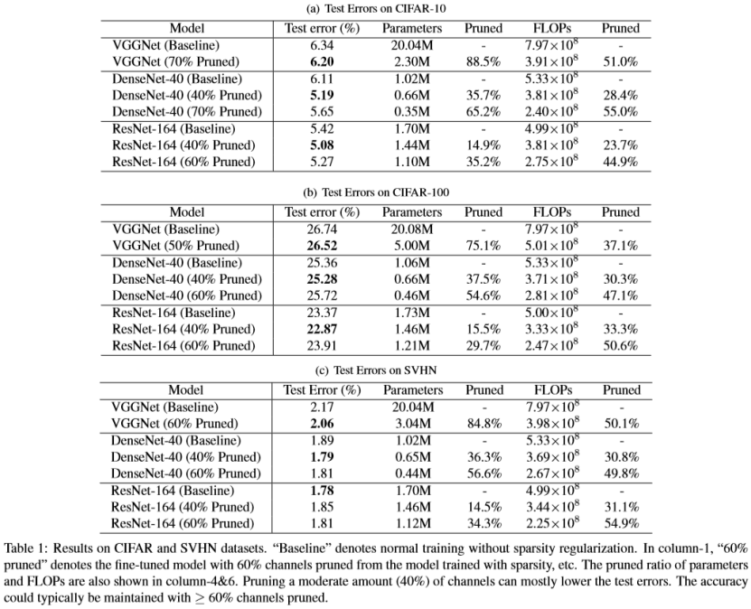
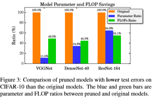
Parameter and FLOP reductions. The purpose of network slimming is to reduce the amount of computing resources needed. The last row of each model has ≥ 60% channels pruned while still maintaining similar accuracy to the baseline. The parameter saving can be up to 10×. The FLOP reductions are typically around 50%. To highlight network slimming’s efficiency, we plot the resource savings in Figure 3. It can be observed that VGGNet has a large amount of redundant parameters that can be pruned. On ResNet-164 the parameter and FLOP savings are relatively insignificant, we conjecture this is due to its “bottleneck” structure has already functioned as selecting channels. Also, on CIFAR-100 the reduction rate is typically slightly lower than CIFAR-10 and SVHN, which is possibly due to the fact that CIFAR-100 contains more classes.
参数和FLOP减少。 网络瘦身的目的是减少所需的计算资源量。 每个模型的最后一行修剪了≥60%的通道,同时仍然保持与基线相似的精度。 参数保存最高可达10倍。 FLOP减少量通常约为50%。 为了突出网络瘦身的效率,我们绘制了图3中的资源节省情况。可以观察到VGGNet具有大量可以修剪的冗余参数。 在ResNet-164上,参数和FLOP节省是相对不重要的,我们推测这是由于其“瓶颈”结构已经起到选择通道的作用。 此外,在CIFAR-100上,降低率通常略低于CIFAR-10和SVHN,这可能是由于CIFAR-100包含更多类。
Regularization Effect. From Table 1, we can observe that, on ResNet and DenseNet, typically when 40% channels are pruned, the fine-tuned network can achieve a lower test error than the original models. For example, DenseNet-40 with 40% channels pruned achieve a test error of 5.19% on CIFAR-10, which is almost 1% lower than the original model. We hypothesize this is due to the regularization effect of L1 sparsity on channels, which naturally provides feature selection in intermediate layers of a network. We will analyze this effect in the next section.
正则化影响。 从表1中我们可以看出,在ResNet和DenseNet上,通常在修剪40%的通道时,经过调整的网络可以实现比原始模型更低的测试误差。 例如,具有40%通道修剪的DenseNet-40在CIFAR-10上实现了5.19%的测试误差,这比原始模型低近1%。 我们假设这是由于L1稀疏性对通道的正则化效应,这自然地在网络的中间层中提供特征选择。 我们将在下一节分析这种效果。
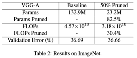
ImageNet. The results for ImageNet dataset are summarized in Table 2. When 50% channels are pruned, the parameter saving is more than 5×, while the FLOP saving is only 30.4%. This is due to the fact that only 378 (out of 2752) channels from all the computation-intensive convolutional layers are pruned, while 5094 neurons (out of 8192) from the parameter-intensive fully-connected layers are pruned. It is worth noting that our method can achieve the savings with no accuracy loss on the 1000-class ImageNet dataset, where other methods for efficient CNNs [2, 23, 35, 28] mostly report accuracy loss.
ImageNet。 ImageNet数据集的结果总结在表2中。当修剪50%通道时,参数节省超过5倍,而FLOP节省仅为30.4%。 这是因为所有计算密集型卷积层中仅有378个(2752个)通道被修剪,而来自参数密集型全连接层的5094个神经元(8192个)被修剪。 值得注意的是,我们的方法可以在1000个类ImageNet数据集上实现节省而没有精度损失,其中有效CNN的其他方法[2,23,35,28]都有报告精度损失。
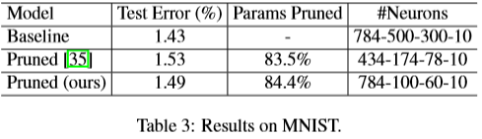
MNIST. On MNIST dataset, we compare our method with the Structured Sparsity Learning (SSL) method [35] in Table 3. Despite our method is mainly designed to prune channels in convolutional layers, it also works well in pruning neurons in fully-connected layers. In this experiment, we observe that pruning with a global threshold sometimes completely removes a layer, thus we prune 80% of the neurons in each of the two intermediate layers. Our method slightly outperforms [35], in that a slightly lower test error is achieved while pruning more parameters.
MNIST。 在MNIST数据集上,我们将我们的方法与表3中的结构化稀疏度学习(SSL)方法[35]进行了比较。尽管我们的方法主要用于修剪卷积层中的通道,但它也可以很好地修剪完全连接层中的神经元。 在这个实验中,我们观察到用全局阈值修剪有时会完全去除一层,因此我们修剪了两个中间层中每个中80%的神经元。 我们的方法稍微优于[35],因为在修剪更多参数时实现了略低的测试误差。
We provide some additional experimental results in the supplementary materials, including (1) detailed structure of a compact VGGNet on CIFAR-10; (2) wall-clock time and run-time memory savings in practice. (3) comparison with a previous channel pruning method [23];
我们在补充材料中提供了一些额外的实验结果,包括(1)CIFAR-10上紧凑型VGGNet的详细结构; (2)在实践中节省挂钟时间(怎么翻译?加载时间?)和运行时间。 (3)与以前的通道修剪方法[23]进行比较;
4.5. Results for Multi-pass Scheme
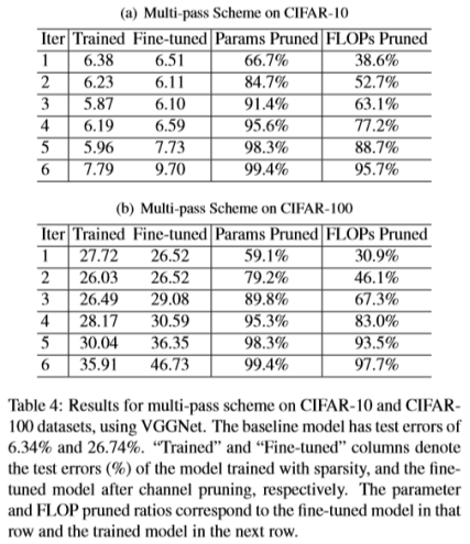
We employ the multi-pass scheme on CIFAR datasets using VGGNet. Since there are no skip-connections, pruning away a whole layer will completely destroy the models. Thus, besides setting the percentile threshold as 50%, we also put a constraint that at each layer, at most 50% of channels can be pruned.
我们在使用VGGNet的CIFAR数据集上采用多程方案。 由于没有跳跃连接,修剪整个层将完全破坏模型。 因此,除了将百分位数阈值设置为50%之外,我们还设置了一个约束,即在每一层,最多可以修剪50%的通道。
The test errors of models in each iteration are shown in Table 4. As the pruning process goes, we obtain more and more compact models. On CIFAR-10, the trained model achieves the lowest test error in iteration 5. This model achieves 20× parameter reduction and 5× FLOP reduction, while still achieving lower test error. On CIFAR-100, after iteration 3, the test error begins to increase. This is possibly due to that it contains more classes than CIFAR-10, so pruning channels too agressively will inevitably hurt the performance. However, we can still prune near 90% parameters and near 70% FLOPs without notable accuracy loss.
每次迭代中模型的测试误差如表4所示。随着修剪过程的进行,我们获得了越来越紧凑的模型。 在CIFAR-10上,经过训练的模型在迭代5次实现了最低的测试误差。该模型实现了20倍的参数减少和5×FLOP减少,同时仍然实现了较低的测试误差。 在CIFAR-100上,在迭代3次之后,测试误差开始增加。 这可能是因为它包含比CIFAR-10更多的类,因此修剪频道过于激进将不可避免地损害性能。 然而,我们仍然可以修剪接近90%的参数和接近70%的FLOP而没有明显的精度损失。
5. Analysis
There are two crucial hyper-parameters in network slimming, the pruned percentage t and the coefficient of the sparsity regularization term λ (see Equation 1). In this section, we analyze their effects in more detail.
网络瘦身有两个关键的超参数,修剪百分比t和稀疏正则化项λ的系数(见公式1)。 在本节中,我们将更详细地分析它们的影响。
Effect of Pruned Percentage. Once we obtain a model trained with sparsity regularization, we need to decide what percentage of channels to prune from the model. If we prune too few channels, the resource saving can be very limited. However, it could be destructive to the model if we prune too many channels, and it may not be possible to recover the accuracy by fine-tuning. We train a DenseNet40 model with λ=10−5 on CIFAR-10 to show the effect of pruning a varying percentage of channels. The results are summarized in Figure 5.
修剪百分比的影响。 一旦我们获得了通过稀疏正则化训练的模型,我们需要确定从模型中修剪的通道百分比。 如果我们修剪太少的频道,节省的资源可能会非常有限。 然而,如果我们修剪太多通道,它可能对模型具有破坏性,并且可能无法通过微调来恢复精度。 我们在CIFAR-10上训练一个λ= 10-5的DenseNet40模型,以显示修剪不同百分比通道的效果。 结果总结在图5中。
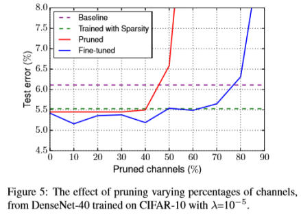
From Figure 5, it can be concluded that the classification performance of the pruned or fine-tuned models degrade only when the pruning ratio surpasses a threshold. The fine tuning process can typically compensate the possible accuracy loss caused by pruning. Only when the threshold goes beyond 80%, the test error of fine-tuned model falls behind the baseline model. Notably, when trained with sparsity, even without fine-tuning, the model performs better than the original model. This is possibly due the the regularization effect of L1 sparsity on channel scaling factors.
从图5中可以得出结论,修剪或调整后的模型的分类性能仅在修剪比超过阈值时才会降低。 精细调整过程通常可以补偿由修剪引起的可能的精度损失。 只有当阈值超过80%时,精细模型的测试误差才会落后于基线模型。 值得注意的是,当训练有稀疏化时,即使没有进行微调,该模型也比原始模型表现更好。 这可能是由于L1稀疏化对信道缩放因子的正则化效应。
Channel Sparsity Regularization. The purpose of the L1 sparsity term is to force many of the scaling factors to be near zero. The parameter λ in Equation 1 controls its significance compared with the normal training loss. In Figure 4 we plot the distributions of scaling factors in the whole network with different λ values. For this experiment we use a VGGNet trained on CIFAR-10 dataset.
通道稀疏性正规化。 L1稀疏项的目的是迫使许多缩放因子接近零。 等式1中的参数λ控制其与正常训练损失相比的显着性。 在图4中,我们绘制了具有不同λ值的整个网络中缩放因子的分布。 对于本实验,我们使用在CIFAR-10数据集上训练的VGGNet。
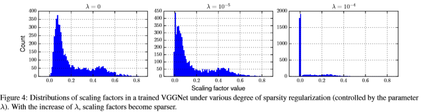
It can be observed that with the increase of λ, the scaling factors are more and more concentrated near zero. When λ=0, i.e., there’s no sparsity regularization, the distribution is relatively flat. When λ=10−4, almost all scaling factors fall into a small region near zero. This process can be seen as a feature selection happening in intermediate layers of deep networks, where only channels with non-negligible scaling factors are chosen. We further visualize this process by a heatmap. Figure 6 shows the magnitude of scaling factors from one layer in VGGNet, along the training process. Each channel starts with equal weights; as the training progresses, some channels’ scaling factors become larger (brighter) while others become smaller (darker).
可以观察到,随着λ的增加,比例因子越来越集中在零附近。 当λ= 0时,即没有稀疏正则化时,分布相对较小。 当λ= 10-4时,几乎所有比例因子都落入接近零的小区域。 该过程可被视为在深度网络的中间层中发生的特征选择,其中仅选择具有不可忽略的缩放因子的通道。 我们通过热图进一步可视化此过程。 图6显示了VGGNet中沿着训练过程的一个层的缩放因子的大小。 每个通道以相同的权重开始; 随着训练的进行,一些频道的缩放因子变得更大(更亮),而其他频道变得更小(更暗)。

6. Conclusion
We proposed the network slimming technique to learn more compact CNNs. It directly imposes sparsity-induced regularization on the scaling factors in batch normalization layers, and unimportant channels can thus be automatically identified during training and then pruned. On multiple datasets, we have shown that the proposed method is able to significantly decrease the computational cost (up to 20×) of state-of-the-art networks, with no accuracy loss. More importantly, the proposed method simultaneously reduces the model size, run-time memory, computing operations while introducing minimum overhead to the training process, and the resulting models require no special libraries/hardware for efficient inference.
我们提出了网络瘦身技术来学习更紧凑的CNN。 它直接对批量归一化层中的缩放因子施加稀疏诱导的正则化,因此可以在训练期间自动识别不重要的通道,然后进行修剪。 在多个数据集上,我们已经表明,所提出的方法能够显着降低最先进网络的计算成本(高达20倍),没有精度损失。 更重要的是,所提出的方法同时减少了模型大小,运行时内存,计算操作,同时为训练过程引入了最小的开销,并且所得到的模型不需要特殊的库/硬件来进行有效的推理。
References
[1] B. Baker, O. Gupta, N. Naik, and R. Raskar. Designing neural network architectures using reinforcement learning. In ICLR, 2017.
[2] S. Changpinyo, M. Sandler, and A. Zhmoginov. The power of sparsity in convolutional neural networks. arXiv preprint arXiv:1702.06257, 2017.
[3] W. Chen, J. T. Wilson, S. Tyree, K. Q. Weinberger, and Y. Chen. Compressing neural networks with the hashing trick. In ICML, 2015.
[4] S. Chintala. Training an object classifier in torch-7 on multiple gpus over imagenet. https://github.com/ soumith/imagenet-multiGPU.torch.
[5] R. Collobert, K. Kavukcuoglu, and C. Farabet. Torch7: A matlab-like environment for machine learning. In BigLearn, NIPS Workshop, number EPFL-CONF-192376, 2011.
[6] M. Courbariaux and Y. Bengio. Binarynet: Training deep neural networks with weights and activations constrained to+ 1 or-1. arXiv preprint arXiv:1602.02830, 2016.
[7] E. L. Denton, W. Zaremba, J. Bruna, Y. LeCun, and R. Fergus. Exploiting linear structure within convolutional networks for efficient evaluation. In NIPS, 2014.
[8] R. Girshick, J. Donahue, T. Darrell, and J. Malik. Rich feature hierarchies for accurate object detection and semantic segmentation. In CVPR, pages 580–587, 2014.
[9] I. Goodfellow, D. Warde-Farley, M. Mirza, A. Courville, and Y. Bengio. Maxout networks. In ICML, 2013.
[10] S. Gross and M. Wilber. Training and investigating residual nets. https://github.com/szagoruyko/cifar. torch.
[11] S. Han, H. Mao, and W. J. Dally. Deep compression: Compressing deep neural network with pruning, trained quantization and huffman coding. In ICLR, 2016.
[12] S. Han, J. Pool, J. Tran, and W. Dally. Learning both weights and connections for efficient neural network. In NIPS, pages 1135–1143, 2015.
[13] K. He, X. Zhang, S. Ren, and J. Sun. Delving deep into rectifiers: Surpassing human-level performance on imagenet classification. In ICCV, 2015.
[14] K. He, X. Zhang, S. Ren, and J. Sun. Deep residual learning for image recognition. In CVPR, 2016.
[15] K. He, X. Zhang, S. Ren, and J. Sun. Identity mappings in deep residual networks. In ECCV, pages 630–645. Springer, 2016.
[16] G. Huang, D. Chen, T. Li, F. Wu, L. van der Maaten, and K. Q. Weinberger. Multi-scale dense convolutional networks for efficient prediction. arXiv preprint arXiv:1703.09844, 2017.
[17] G. Huang, Z. Liu, K. Q. Weinberger, and L. van der Maaten. Densely connected convolutional networks. In CVPR, 2017.
[18] G. Huang, Y. Sun, Z. Liu, D. Sedra, and K. Q. Weinberger. Deep networks with stochastic depth. In ECCV, 2016.
[19] S. Ioffe and C. Szegedy. Batch normalization: Accelerating deep network training by reducing internal covariate shift. arXiv preprint arXiv:1502.03167, 2015.
[20] J. Jin, Z. Yan, K. Fu, N. Jiang, and C. Zhang. Neural network architecture optimization through submodularity and supermodularity. arXiv preprint arXiv:1609.00074, 2016.
[21] A. Krizhevsky and G. Hinton. Learning multiple layers of features from tiny images. In Tech Report, 2009.
[22] A. Krizhevsky, I. Sutskever, and G. E. Hinton. Imagenet classification with deep convolutional neural networks. In NIPS, pages 1097–1105, 2012.
[23] H. Li, A. Kadav, I. Durdanovic, H. Samet, and H. P. Graf. Pruning filters for efficient convnets. arXiv preprint arXiv:1608.08710, 2016.
[24] M. Lin, Q. Chen, and S. Yan. Network in network. In ICLR, 2014.
[25] B. Liu, M. Wang, H. Foroosh, M. Tappen, and M. Pensky. Sparse convolutional neural networks. In Proceedings of the IEEE Conference on Computer Vision and Pattern Recognition, pages 806–814, 2015.
[26] J. Long, E. Shelhamer, and T. Darrell. Fully convolutional networks for semantic segmentation. In CVPR, pages 3431– 3440, 2015.
[27] Y. Netzer, T. Wang, A. Coates, A. Bissacco, B. Wu, and A. Y. Ng. Reading digits in natural images with unsupervised feature learning, 2011. In NIPS Workshop on Deep Learning and Unsupervised Feature Learning, 2011.
[28] M. Rastegari, V. Ordonez, J. Redmon, and A. Farhadi. Xnornet: Imagenet classification using binary convolutional neural networks. In ECCV, 2016.
[29] S. Scardapane, D. Comminiello, A. Hussain, and A. Uncini. Group sparse regularization for deep neural networks. arXiv preprint arXiv:1607.00485, 2016.
[30] M. Schmidt, G. Fung, and R. Rosales. Fast optimization methods for l1 regularization: A comparative study and two new approaches. In ECML, pages 286–297, 2007.
[31] K. Simonyan and A. Zisserman. Very deep convolutional networks for large-scale image recognition. In ICLR, 2015.
[32] S. Srinivas, A. Subramanya, and R. V. Babu. Training sparse neural networks. CoRR, abs/1611.06694, 2016.
[33] I. Sutskever, J. Martens, G. Dahl, and G. Hinton. On the importance of initialization and momentum in deep learning. In ICML, 2013.
[34] C. Szegedy, W. Liu, Y. Jia, P. Sermanet, S. Reed, D. Anguelov, D. Erhan, et al. Going deeper with convolutions. In CVPR, pages 1–9, 2015.
[35] W. Wen, C. Wu, Y. Wang, Y. Chen, and H. Li. Learning structured sparsity in deep neural networks. In NIPS, 2016.
[36] S. Zagoruyko. 92.5% on cifar-10 in torch. https:// github.com/szagoruyko/cifar.torch.
[37] H.Zhou, J.M.Alvarez, andF.Porikli. Lessismore: Towards compact cnns. In ECCV, 2016.
[38] B. Zoph and Q. V. Le. Neural architecture search with reinforcement learning. In ICLR, 2017.