Deep Neural Network for Image Classification: Application(深度神经网络在图像分类中的应用)
本文作业是在jupyter notebook上一步一步做的,带有一些过程中查找的资料等(出处已标明)并翻译成了中文,如有错误,欢迎指正!
当你完成这个,你就完成了第四周的最后一个编程作业,也是这门课的最后一个编程作业!
您将使用在上一个任务中实现的函数来构建深度网络,并将其应用于cat和非cat分类。希望您能看到相对于以前的逻辑回归实现,准确度有所提高。
完成这项任务后,您将能够:
•建立和应用深度神经网络来监督学习。
让我们开始吧!
1 - Packages 包
•numpy是使用Python进行科学计算的基本包。
•matplotlib是一个用Python绘制图形的库。
•h5py是与存储在H5文件上的数据集交互的常用包。
•PIL和scipy在这里用你自己的图片测试你的模型。
•dnn_app_utils提供了在“构建深层神经网络:一步一步”任务中实现的函数。也就是上一节我们所做的函数
•seed(1)用于保持所有随机函数调用的一致性。它将帮助我们批改你的作业。
 1 import time
 2 import numpy as np
 3 import h5py
 4 import matplotlib.pyplot as plt
 5 import scipy
 6 from PIL import Image
 7 from scipy import ndimage
 8 from dnn_app_utils_v2 import *
 9
10 %matplotlib inline
11 plt.rcParams['figure.figsize'] = (5.0, 4.0) # set default size of plots
12 plt.rcParams['image.interpolation'] = 'nearest'
13 plt.rcParams['image.cmap'] = 'gray'
14
15 %load_ext autoreload
16 %autoreload 2
17
18 np.random.seed(1)
%load_ext autoreload自动加载 来自:熊熊的小心心
2 - Dataset 数据集
你将使用与“逻辑回归作为神经网络”(作业2)中相同的“猫和非猫”数据集。你所建立的模型在对猫和非猫图像进行分类方面有70%的测试准确率。希望您的新模型能表现得更好!
问题陈述:给你一个数据集(“data.h5”),包含:
-标记为cat(1)或non-cat(0)的m_train图像的训练集
- m_test图像标记为猫和非猫的测试集
-每个图像是形状(num_px, num_px, 3),其中3是3通道(RGB)。
让我们更加熟悉数据集。通过运行下面的单元格加载数据。
train_x_orig, train_y, test_x_orig, test_y, classes = load_data()
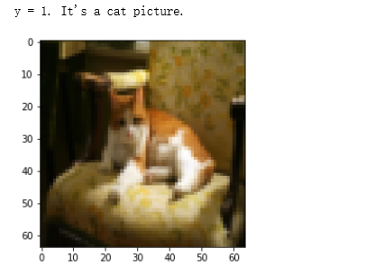
下面的代码将显示数据集中的映像。您可以随意更改索引并多次重新运行单元格以查看其他图像。(一共有209张照片)
# Example of a picture
index = 7
plt.imshow(train_x_orig[index])
print ("y = " + str(train_y[0,index]) + ". It's a " + classes[train_y[0,index]].decode("utf-8") +  " picture.")
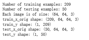
# Explore your dataset
m_train = train_x_orig.shape[0]
num_px = train_x_orig.shape[1]
m_test = test_x_orig.shape[0]

print ("Number of training examples: " + str(m_train))
print ("Number of testing examples: " + str(m_test))
print ("Each image is of size: (" + str(num_px) + ", " + str(num_px) + ", 3)")
print ("train_x_orig shape: " + str(train_x_orig.shape))
print ("train_y shape: " + str(train_y.shape))
print ("test_x_orig shape: " + str(test_x_orig.shape))
print ("test_y shape: " + str(test_y.shape))
像往常一样,在将图像提供给网络之前,需要对它们进行重塑和标准化。代码在下面的单元格中给出。
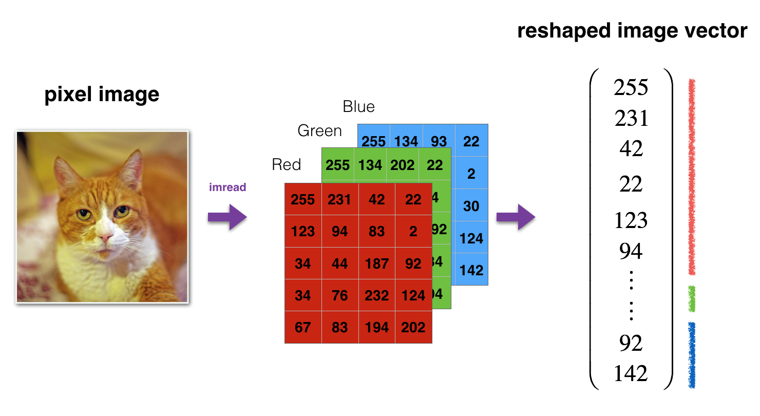
Figure 1: Image to vector conversion.(图1:图像到矢量的转换。)
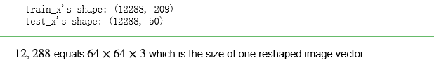
# Reshape the training and test examples
train_x_flatten = train_x_orig.reshape(train_x_orig.shape[0], -1).T   # The "-1" makes reshape flatten the remaining dimensions
test_x_flatten = test_x_orig.reshape(test_x_orig.shape[0], -1).T    #“-1”使重塑压平剩余的维度

# Standardize data to have feature values between 0 and 1. 对数据进行标准化,使其特征值在0到1之间。 因为RGB值最大就是255
train_x = train_x_flatten/255.
test_x = test_x_flatten/255.

print ("train_x's shape: " + str(train_x.shape))
print ("test_x's shape: " + str(test_x.shape))
结果:
3 - Architecture of your model (模型的架构)
现在您已经熟悉了数据集,现在可以构建一个深度神经网络来区分cat图像和非cat图像了。
您将构建两个不同的模型:
A 2-layer neural network 一个2层神经网络
An L-layer deep neural network 一个L层深度神经网络
然后您将比较这些模型的性能,并为 L尝试不同的值。
让我们看看这两种架构。
3.1 - 2-layer neural network 二层的神经网络
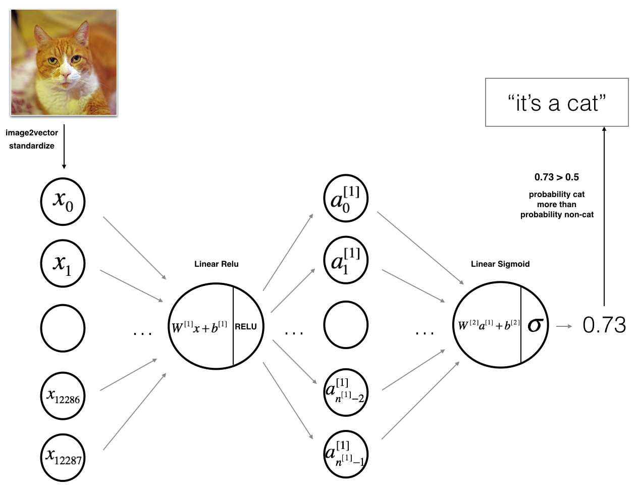
Figure 2: 2-layer neural network. 图2 2层的神经网络
The model can be summarized as: ***INPUT -> LINEAR -> RELU -> LINEAR -> SIGMOID -> OUTPUT***.
图2的详细架构:
•输入是一个(64,64,3)图像,它被平展成一个大小为矢量(12288,1)的图像。
•对应向量:[x 0,x 1,…x12287]T乘以大小为(n[1],12288)的权值矩阵W[1]。
•添加一个偏差项,取其relu得到以下向量:[a [1] 0,a[1] 1,…,a [1] n[1]−1]T。
•然后重复同样的过程。
•将得到的向量乘以W[2],并加上截距(偏置)。
•最后,取结果的sigmoid。如果它大于0.5,你就把它归类为猫。
3.2 - L-layer deep neural network L层深度神经网络
用上述表示方法来表示一个L层深度神经网络是很困难的。但是,这里有一个简化的网络表示:
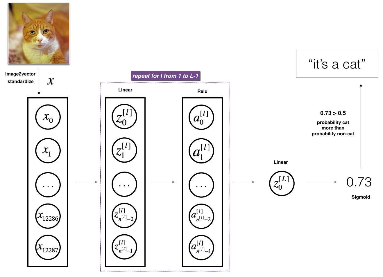
Figure 3: L-layer neural network. 图3 L层神经网络
The model can be summarized as: ***[LINEAR -> RELU]
图3的详细架构:
•输入是一个(64,64,3)图像,它被平展成一个大小为矢量(12288,1)的图像。
•对应向量:[x 0,x 1,…x12287]T乘以权重矩阵W,然后加上截距b。其结果称为线性单元。
•接下来,取线性单位的relu。根据模型架构的不同,这个过程可以为每个(W [l],b [l])重复几次。
•最后,取最后一个线性单位的sigmoid。如果它大于0.5,你就把它归类为猫。
3.3 - General methodology 一般方法
和往常一样,你将遵循深度学习的方法来构建模型:
1. 初始化参数/定义超参数
2. num_iterations循环:
a.一个向前传播。
b.计算成本函数
c.反向传播
d.更新参数(使用参数和从backprop获得的梯度)
3. 使用训练过的参数来预测标签
现在让我们实现这两个模型!
4 - Two-layer neural network 2层神经网络
问:使用您在前一个任务中实现的辅助函数来构建一个2层神经网络,其结构如下:LINEAR -> RELU -> LINEAR -> SIGMOID。你可能需要的功能和它们的输入是:
def initialize_parameters(n_x, n_h, n_y):
    ...
    return parameters
def linear_activation_forward(A_prev, W, b, activation):
    ...
    return A, cache
def compute_cost(AL, Y):
    ...
    return cost
def linear_activation_backward(dA, cache, activation):
    ...
    return dA_prev, dW, db
def update_parameters(parameters, grads, learning_rate):
    ...
    return parameters
### CONSTANTS DEFINING THE MODEL ####定义模型的常量
n_x = 12288     # num_px * num_px * 3 (64 X 64 X 3)
n_h = 7  #隐藏层的单元数有7个
n_y = 1  #输出一个标签值
layers_dims = (n_x, n_h, n_y)  #层的形状


 1 # GRADED FUNCTION: two_layer_model
 2
 3 def two_layer_model(X, Y, layers_dims, learning_rate = 0.0075, num_iterations = 3000, print_cost=False):
 4     """
 5     Implements a two-layer neural network: LINEAR->RELU->LINEAR->SIGMOID.实现一个2层的神经网络
 6
 7     Arguments(参数):
 8     X -- input data, of shape (n_x, number of examples) 输入的数据,形状是(n_x, 样本数量)
 9     Y -- true "label" vector (containing 0 if cat, 1 if non-cat), of shape (1, number of examples)
10     layers_dims -- dimensions of the layers (n_x, n_h, n_y)
11     num_iterations -- number of iterations of the optimization loop (优化循环迭代的次数)
12     learning_rate -- learning rate of the gradient descent update rule
13     print_cost -- If set to True, this will print the cost every 100 iterations 每迭代100次打印一次成本
14
15     Returns:
16     parameters -- a dictionary containing W1, W2, b1, and b2  返回的是一个字典,包含了 W1, W2, b1 和 b2
17     """
18
19     np.random.seed(1)
20     grads = {}
21     costs = []                              # to keep track of the cost 记录成本
22     m = X.shape[1]                           # number of examples 样本的数量
23     (n_x, n_h, n_y) = layers_dims
24
25     # Initialize parameters dictionary, by calling one of the functions you'd previously implemented
26     ### START CODE HERE ### (≈ 1 line of code)
27     parameters = initialize_parameters(n_x, n_h, n_y, )
28     ### END CODE HERE ###
29
30     # Get W1, b1, W2 and b2 from the dictionary parameters.
31     W1 = parameters["W1"]
32     b1 = parameters["b1"]
33     W2 = parameters["W2"]
34     b2 = parameters["b2"]
35
36     # Loop (gradient descent)
37
38     for i in range(0, num_iterations):
39
40         # Forward propagation: LINEAR -> RELU -> LINEAR -> SIGMOID. Inputs: "X, W1, b1". Output: "A1, cache1, A2, cache2".
41         ### START CODE HERE ### (≈ 2 lines of code)
42         A1, cache1 = linear_activation_forward(X, W1, b1, activation = "relu")
43         A2, cache2 = linear_activation_forward(A1, W2, b2, activation = "sigmoid")
44         ### END CODE HERE ###
45
46         # Compute cost
47         ### START CODE HERE ### (≈ 1 line of code)
48         cost = compute_cost(A2, Y)
49         ### END CODE HERE ###
50
51         # Initializing backward propagation
52         dA2 = - (np.divide(Y, A2) - np.divide(1 - Y, 1 - A2))
53
54         # Backward propagation. Inputs: "dA2, cache2, cache1". Outputs: "dA1, dW2, db2; also dA0 (not used), dW1, db1".
55         ### START CODE HERE ### (≈ 2 lines of code)
56         dA1, dW2, db2 = linear_activation_backward(dA2, cache2, activation = "sigmoid")
57         dA0, dW1, db1 = linear_activation_backward(dA1, cache1, activation = "relu")
58         ### END CODE HERE ###
59
60         # Set grads['dWl'] to dW1, grads['db1'] to db1, grads['dW2'] to dW2, grads['db2'] to db2
61         grads['dW1'] = dW1
62         grads['db1'] = db1
63         grads['dW2'] = dW2
64         grads['db2'] = db2
65
66         # Update parameters.
67         ### START CODE HERE ### (approx. 1 line of code)
68         parameters = update_parameters(parameters, grads, learning_rate)
69         ### END CODE HERE ###
70
71         # Retrieve W1, b1, W2, b2 from parameters 从参数中检索W1、b1、W2、b2
72         W1 = parameters["W1"]
73         b1 = parameters["b1"]
74         W2 = parameters["W2"]
75         b2 = parameters["b2"]
76
77         # Print the cost every 100 training example 每100次训练样本打印一次成本
78         if print_cost and i % 100 == 0:
79             print("Cost after iteration {}: {}".format(i, np.squeeze(cost))) #从数组的形状中删除单维度条目,即把shape中为1的维度去掉
80         if print_cost and i % 100 == 0:
81             costs.append(cost)
82
83     # plot the cost 图示成本
84
85     plt.plot(np.squeeze(costs))
86     plt.ylabel('cost')
87     plt.xlabel('iterations (per tens)')
88     plt.title("Learning rate =" + str(learning_rate))
89     plt.show()
90
91     return parameters
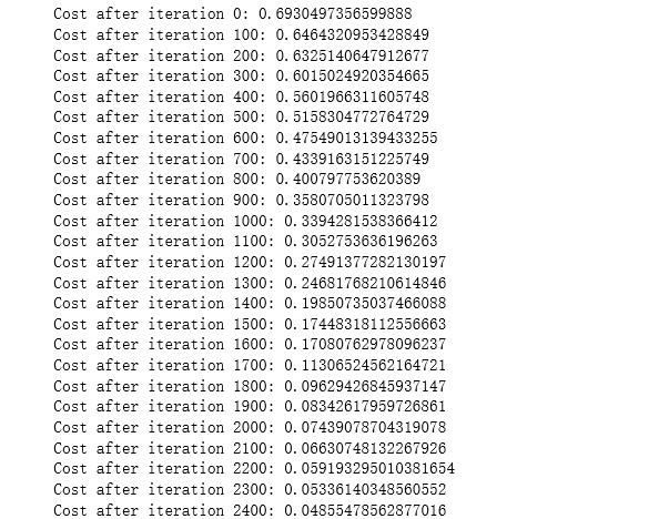
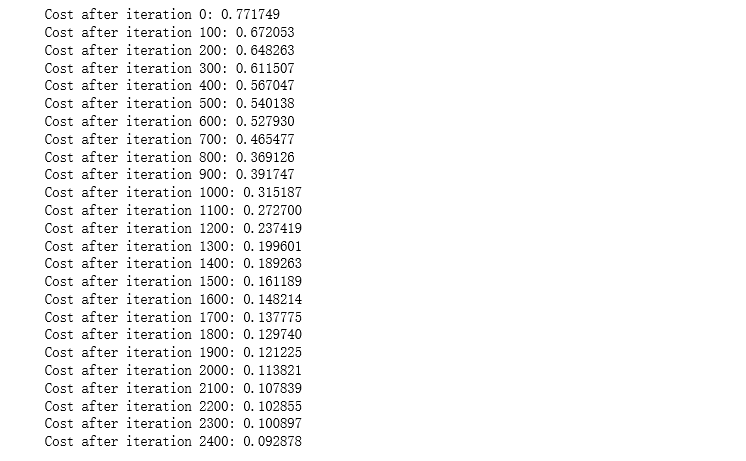
运行下面的单元来训练参数。看看您的模型是否运行。成本应该会降低。运行2500次迭代可能需要5分钟。检查迭代0”后“成本与预期的输出匹配,如果不点击广场(⬛)上酒吧的笔记本停止细胞,试图找到你的错误。
parameters = two_layer_model(train_x, train_y, layers_dims = (n_x, n_h, n_y), num_iterations = 2500, print_cost=True)

幸好您构建了一个向量化的实现!否则可能要花10倍的时间来训练它。
现在,您可以使用经过训练的参数对数据集中的图像进行分类。要查看对训练集和测试集的预测,请运行下面的单元。
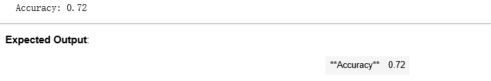
predictions_train = predict(train_x, train_y, parameters)
结果:
predictions_test = predict(test_x, test_y, parameters)
#这个predict()函数是写好的吗?
结果:
注意:您可能注意到在更少的迭代(比如1500次)上运行模型可以在测试集上提供更好的准确性。这被称为“早期停止”,我们将在下一课中讨论它。提前停止是防止过拟合的一种方法。
恭喜你!看起来你的两层神经网络比逻辑回归实现(70%,作业周2)有更好的性能(72%)。
5 - L-layer Neural Network L层的神经网络
问题:使用您之前实现的辅助函数来构建一个结构如下的L层神经网络:[LINEAR -> RELU] * (L-1) -> LINEAR -> SIGMOID。你可能需要的功能和它们的输入是:
def initialize_parameters_deep(layer_dims):
    ...
    return parameters
def L_model_forward(X, parameters):
    ...
    return AL, caches
def compute_cost(AL, Y):
    ...
    return cost
def L_model_backward(AL, Y, caches):
    ...
    return grads
def update_parameters(parameters, grads, learning_rate):
    ...
    return parameters
### CONSTANTS ###常量
layers_dims = [12288, 20, 7, 5, 1] #  5-layer model 这里我的理解是每层的单元数,第0层是64*64*3,第1~3层是隐藏层,单元数分别是20,7,5,第4层就是输出层了
 1 # GRADED FUNCTION: L_layer_model
 2
 3 def L_layer_model(X, Y, layers_dims, learning_rate = 0.0075, num_iterations = 3000, print_cost=False):#lr was 0.009
 4     """
 5     Implements a L-layer neural network: [LINEAR->RELU]*(L-1)->LINEAR->SIGMOID.最后一层的激活函数是sigmoid
 6
 7     Arguments:
 8     X -- data, numpy array of shape (number of examples, num_px * num_px * 3)这里为啥把样本数放前面了?个人认为是解释标反了
 9     Y -- true "label" vector (containing 0 if cat, 1 if non-cat), of shape (1, number of examples)
10     layers_dims -- list containing the input size and each layer size, of length (number of layers + 1).
11     learning_rate -- learning rate of the gradient descent update rule
12     num_iterations -- number of iterations of the optimization loop
13     print_cost -- if True, it prints the cost every 100 steps
14
15     Returns:
16     parameters -- parameters learnt by the model. They can then be used to predict.
17     """
18
19     np.random.seed(1)
20     costs = []                         # keep track of cost
21
22     # Parameters initialization.参数的初始化
23     ### START CODE HERE ###
24     parameters = initialize_parameters_deep(layers_dims)
25     ### END CODE HERE ###
26
27     # Loop (gradient descent) 循环(梯度下降) 这边少不了一个显示的for循环,避免不了
28     for i in range(0, num_iterations):
29
30         # Forward propagation: [LINEAR -> RELU]*(L-1) -> LINEAR -> SIGMOID.
31         ### START CODE HERE ### (≈ 1 line of code)
32         AL, caches = L_model_forward(X, parameters)
33         ### END CODE HERE ###
34
35         # Compute cost.
36         ### START CODE HERE ### (≈ 1 line of code)
37         cost = compute_cost(AL, Y)
38         ### END CODE HERE ###
39
40         # Backward propagation.
41         ### START CODE HERE ### (≈ 1 line of code)
42         grads = L_model_backward(AL, Y, caches)
43         ### END CODE HERE ###
44
45         # Update parameters.参数更新
46         ### START CODE HERE ### (≈ 1 line of code)
47         parameters = update_parameters(parameters, grads, learning_rate)
48         ### END CODE HERE ###
49
50         # Print the cost every 100 training example 每100次训练样本,打印一次成本
51         if print_cost and i % 100 == 0:
52             print ("Cost after iteration %i: %f" %(i, cost))
53         if print_cost and i % 100 == 0:
54             costs.append(cost)
55
56     # plot the cost
57     plt.plot(np.squeeze(costs))
58     plt.ylabel('cost')
59     plt.xlabel('iterations (per tens)')
60     plt.title("Learning rate =" + str(learning_rate))
61     plt.show()
62
63     return parameters
现在,您将把模型训练成一个5层神经网络。
运行下面的单元来训练你的模型。每次迭代的成本都应该降低。运行2500次迭代可能需要5分钟。检查迭代0”后“成本与预期的输出匹配,如果不点击广场(⬛)上酒吧的笔记本停止细胞,试图找到你的错误。
parameters = L_layer_model(train_x, train_y, layers_dims, num_iterations = 2500, print_cost = True)
结果:

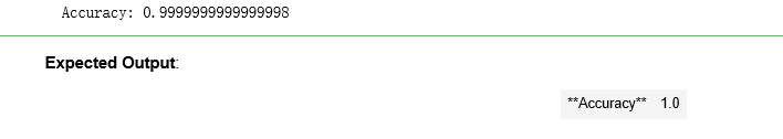
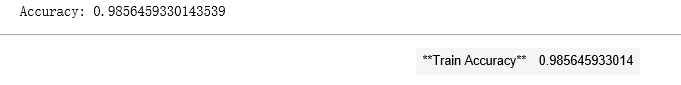
pred_train = predict(train_x, train_y, parameters)
结果:
pred_test = predict(test_x, test_y, parameters)
结果:
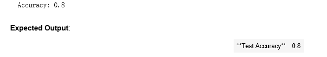
恭喜!在相同的测试集上,5层神经网络的性能(80%)似乎比2层神经网络的性能(72%)要好。
对于这项任务来说,这是很好的表现。不错的工作!
在下一节关于“改进深度神经网络”的课程中,您将学习如何通过系统地搜索更好的超参数(learning_rate、layers_dims、num_iterations,以及其他您将在下一节课程中学习的超参数)来获得更高的精度。
6) Results Analysis 结果分析
首先,让我们看一些图片的L-layer模型标签不正确。这将显示一些标签错误的图像。
print_mislabeled_images(classes, test_x, test_y, pred_test)
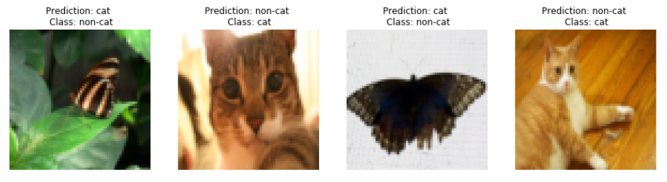
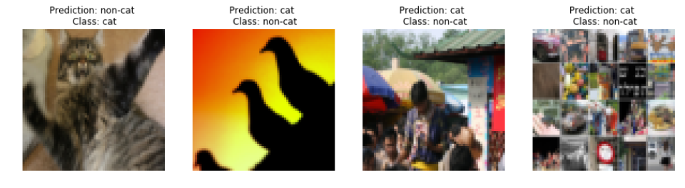

一些类型的图像模型往往做得不好,包括:
•猫的身体处于不寻常的位置
•猫出现在相似颜色的背景上
•不寻常的猫的颜色和种类
•相机角度
•图片的亮度
•尺度变化(cat在图像中非常大或很小)
7) Test with your own image (optional/ungraded exercise) 用自己的图像测试(可选/未分级练习)
恭喜你完成了这项任务。您可以使用自己的图像并查看模型的输出。这样做:
1. 点击笔记本上端的“文件”,然后点击“打开”进入Coursera中心。
2. 将您的图像添加到此木星笔记本的目录,在“images”文件夹中
3.在下面的代码中更改映像的名称
4. 运行代码并检查算法是否正确(1 = cat, 0 = non-cat)!
会报警:

## START CODE HERE ##
my_image = "tree.jpg" # change this to the name of your image file
my_label_y = [1] # the true class of your image (1 -> cat, 0 -> non-cat)
## END CODE HERE ##

fname = "images/" + my_image
image = np.array(ndimage.imread(fname, flatten=False))
my_image = scipy.misc.imresize(image, size=(num_px,num_px)).reshape((num_px*num_px*3,1))
my_predicted_image = predict(my_image, my_label_y, parameters)

plt.imshow(image)
print ("y = " + str(np.squeeze(my_predicted_image)) + ", your L-layer model predicts a "" + classes[int(np.squeeze(my_predicted_image)),].decode("utf-8") +  "" picture.")
结果:
