python机器学习实战（二）

python机器学习实战（二）
python机器学习实战（二）

版权声明：本文为博主原创文章，转载请指明转载地址

http://www.cnblogs.com/fydeblog/p/7159775.html

前言

这篇notebook是关于机器学习监督学习中的决策树算法，内容包括决策树算法的构造过程，使用matplotlib库绘制树形图以及使用决策树预测隐形眼睛类型.
操作系统：ubuntu14.04（win也ok）运行环境：anaconda-python2.7-jupyter notebook 参考书籍：机器学习实战和源码 notebook writer ----方阳

注意事项：在这里说一句，默认环境python2.7的notebook，用python3.6的会出问题，还有我的目录可能跟你们的不一样，你们自己跑的时候记得改目录，我会把notebook和代码以及数据集放到结尾的百度云盘，方便你们下载！

决策树原理：不断通过数据集的特征来划分数据集，直到遍历所有划分数据集的属性，或每个分支下的实例都具有相同的分类，决策树算法停止运行。

决策树的优缺点及适用类型
优点 :计算复杂度不高, 输出结果易于理解,对中间值的缺失不敏感,可以处理不相关特征数据。
缺点 :可能会产生过度匹配问题。
适用数据类型:数值型和标称型

先举一个小例子，让你了解决策树是干嘛的，简单来说，决策树算法就是一种基于特征的分类器，拿邮件来说吧，试想一下，邮件的类型有很多种，有需要及时处理的邮件，无聊是观看的邮件，垃圾邮件等等，我们需要去区分这些，比如根据邮件中出现里你的名字还有你朋友的名字，这些特征就会就可以将邮件分成两类，需要及时处理的邮件和其他邮件，这时候在分类其他邮件，例如邮件中出现buy，money等特征，说明这是垃圾推广文件，又可以将其他文件分成无聊是观看的邮件和垃圾邮件了。

1.决策树的构造

1.1 信息增益

试想一下，一个数据集是有多个特征的，我们该从那个特征开始划分呢，什么样的划分方式会是最好的？

我们知道划分数据集的大原则是将无序的数据变得更加有序，这样才能分类得更加清楚，这里就提出了一种概念，叫做信息增益，它的定义是在划分数据集之前之后信息发生的变化，变化越大，证明划分得越好，所以在划分数据集的时候，获得增益最高的特征就是最好的选择。

这里又会扯到另一个概念，信息论中的熵，它是集合信息的度量方式，熵变化越大，信息增益也就越大。信息增益是熵的减少或者是数据无序度的减少.

一个符号x在信息论中的信息定义是 l(x)= -log(p(x)) ,这里都是以2为底，不再复述。

则熵的计算公式是 H =-∑p(xi)log(p(xi)) (i=1,2,..n)

下面开始实现给定数据集，计算熵

参考代码：
```
1 from math import log         #we use log function to calculate the entropy
2 import operator
```
```
 1 def calcShannonEnt(dataSet):
 2     numEntries = len(dataSet)
 3     labelCounts = {}
 4     for featVec in dataSet: #the the number of unique elements and their occurance
 5         currentLabel = featVec[-1]
 6         if currentLabel not in labelCounts.keys(): labelCounts[currentLabel] = 0
 7         labelCounts[currentLabel] += 1
 8     shannonEnt = 0.0
 9     for key in labelCounts:
10         prob = float(labelCounts[key])/numEntries
11         shannonEnt -= prob * log(prob,2)     #log base 2
12     return shannonEnt
```
程序思路：首先计算数据集中实例的总数,由于代码中多次用到这个值,为了提高代码效率,我们显式地声明一个变量保存实例总数. 然后 ,创建一个数据字典labelCounts,它的键值是最后一列（分类的结果）的数值.如果当前键值不存在,则扩展字典并将当前键值加入字典。每个键值都记录了当前类别出现的次数。最后 , 使用所有类标签的发生频率计算类别出现的概率。我们将用这个概率计算香农熵。

让我们来测试一下，先自己定义一个数据集

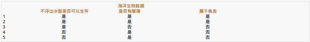
下表的数据包含 5 个海洋动物,特征包括:不浮出水面是否可以生存,以及是否有脚蹼。我们可以将这些动物分成两类: 鱼类和非鱼类。
根据上面的表格，我们可以定义一个createDataSet函数

参考代码如下

1 def createDataSet(): 2 dataSet = [[1, 1, 'yes'], 3 [1, 1, 'yes'], 4 [1, 0, 'no'], 5 [0, 1, 'no'], 6 [0, 1, 'no']] 7 labels = ['no surfacing','flippers'] 8 #change to discrete values 9 return dataSet, labels

把所有的代码都放在trees.py中（以下在jupyter）

cd /home/fangyang/桌面/machinelearninginaction/Ch03

/home/fangyang/桌面/machinelearninginaction/Ch03
```
import trees
```
```
myDat, labels = trees.createDataSet()
```
```
myDat  #old data set
```
```
[[1, 1, 'yes'], [1, 1, 'yes'], [1, 0, 'no'], [0, 1, 'no'], [0, 1, 'no']]
```
labels
['no surfacing', 'flippers']

trees.calcShannonEnt(myDat) #calculate the entropy

0.9709505944546686

myDat[0][-1]='maybe' #change the result ,and look again the entropy

myDat #new data set

[[1, 1, 'maybe'], [1, 1, 'yes'], [1, 0, 'no'], [0, 1, 'no'], [0, 1, 'no']]

trees.calcShannonEnt(myDat) # the new entropy

1.3709505944546687

我们可以看到当结果分类改变，熵也发生里变化，主要是因为最后的结果发生里改变，相应的概率也发生了改变，根据公式，熵也会改变

1.2 划分数据集

前面已经得到了如何去求信息熵的函数，但我们的划分是以哪个特征划分的呢，不知道，所以我们还要写一个以给定特征划分数据集的函数。

参考代码如下：

1 def splitDataSet(dataSet, axis, value): 2 retDataSet = [] 3 for featVec in dataSet: 4 if featVec[axis] == value: 5 reducedFeatVec = featVec[:axis] #chop out axis used for splitting 6 reducedFeatVec.extend(featVec[axis+1:]) 7 retDataSet.append(reducedFeatVec) 8 return retDataSet

函数的三个输人参数:待划分的数据集（dataSet）、划分数据集的特征（axis）、特征的返回值（value）。输出是划分后的数据集（retDataSet）

小知识：python语言在函数中传递的是列表的引用 ,在函数内部对列表对象的修改, 将会影响该列表对象的整个生存周期。为了消除这个不良影响 ,我们需要在函数的开始声明一个新列表对象。因为该函数代码在同一数据集上被调用多次,为了不修改原始数据集,创建一个新的列表对象retDataSet

这个函数也挺简单的，根据axis的值所指的对象来进行划分数据集，比如axis=0，就按照第一个特征来划分，featVec[:axis]就是空,下面经过一个extend函数，将featVec[axis+1:]后面的数存到reduceFeatVec中，然后通过append函数以列表的形式存到retDataSet中。

这里说一下entend和append函数的功能，举个例子吧

a=[1,2,3] b=[4,5,6] a.append(b)

a

[1, 2, 3, [4, 5, 6]]

a=[1,2,3] a.extend(b)

a

[1, 2, 3, 4, 5, 6]
可见append函数是直接将b的原型导入a中，extend是将b中的元素导入到a中
下面再来测试一下

myDat, labels = trees.createDataSet() #initialization

myDat

[[1, 1, 'yes'], [1, 1, 'yes'], [1, 0, 'no'], [0, 1, 'no'], [0, 1, 'no']]

trees.splitDataSet(myDat,0,1) #choose the first character to split the dataset

[[1, 'yes'], [1, 'yes'], [0, 'no']]

trees.splitDataSet(myDat,0,0)# change the value ,look the difference of previous results

[[1, 'no'], [1, 'no']]

好了，我们知道了怎样以某个特征划分数据集了，但我们需要的是最好的数据集划分方式，所以要结合前面两个函数，计算以每个特征为划分方式，相应最后的信息熵，我们要找到最大信息熵，它所对应的特征就是我们要找的最好划分方式。所以有了函数chooseBestFeatureToSpilt

参考代码如下：

1 def chooseBestFeatureToSplit(dataSet): 2 numFeatures = len(dataSet[0]) - 1 #the last column is used for the labels 3 baseEntropy = calcShannonEnt(dataSet) #calculate the original entropy 4 bestInfoGain = 0.0; bestFeature = -1 5 for i in range(numFeatures): #iterate over all the features 6 featList = [example[i] for example in dataSet]#create a list of all the examples of this feature 7 uniqueVals = set(featList) #get a set of unique values 8 newEntropy = 0.0 9 for value in uniqueVals: 10 subDataSet = splitDataSet(dataSet, i, value) 11 prob = len(subDataSet)/float(len(dataSet)) 12 newEntropy += prob * calcShannonEnt(subDataSet) 13 infoGain = baseEntropy - newEntropy #calculate the info gain; ie reduction in entropy 14 if (infoGain > bestInfoGain): #compare this to the best gain so far 15 bestInfoGain = infoGain #if better than current best, set to best 16 bestFeature = i 17 return bestFeature #returns an integer

这个函数就是把前面两个函数整合起来了，先算出特征的数目，由于最后一个是标签，不算特征，所以以数据集长度来求特征数时，要减1。然后求原始的信息熵，是为了跟新的信息熵，进行比较，选出变化最大所对应的特征。这里有一个双重循环，外循环是按特征标号进行循环的，下标从小到大，featList是特征标号对应下的每个样本的值，是一个列表，而uniqueVals是基于这个特征的所有可能的值的集合，内循环做的是以特征集合中的每一个元素作为划分，最后求得这个特征下的平均信息熵，然后原始的信息熵进行比较，得出信息增益，最后的if语句是要找到最大信息增益，并得到最大信息增益所对应的特征的标号。
现在来测试测试
```
import trees
myDat, labels = trees.createDataSet()
trees.chooseBestFeatureToSplit(myDat)   #return the index of best character to split
```
0

1.3 递归构建决策树

好了，到现在，我们已经知道如何基于最好的属性值去划分数据集了，现在进行下一步，如何去构造决策树

决策树的实现原理：得到原始数据集, 然后基于最好的属性值划分数据集,由于特征值可能多于两个,因此可能存在大于两个分支的数据集划分。第一次划分之后, 数据将被向下传递到树分支的下一个节点, 在这个节点上 ,我们可以再次划分数据。因此我们可以采用递归的原则处理数据集。
递归结束的条件是:程序遍历完所有划分数据集的属性, 或者每个分支下的所有实例都具有相同的分类。

这里先构造一个majorityCnt函数，它的作用是返回出现次数最多的分类名称，后面会用到

def majorityCnt(classList): classCount={} for vote in classList: if vote not in classCount.keys(): classCount[vote] = 0 classCount[vote] += 1 sortedClassCount = sorted(classCount.iteritems(), key=operator.itemgetter(1), reverse=True) return sortedClassCount[0][0]

这个函数在实战一中的一个函数是一样的，复述一遍，classCount定义为存储字典，每当，由于后面加了1，所以每次出现键值就加1，就可以就算出键值出现的次数里。最后通过sorted函数将classCount字典分解为列表，sorted函数的第二个参数导入了运算符模块的itemgetter方法，按照第二个元素的次序（即数字）进行排序，由于此处reverse=True，是逆序，所以按照从大到小的次序排列。

让我们来测试一下

import numpy as np classList = np.array(myDat).T[-1]

classList

array(['yes', 'yes', 'no', 'no', 'no'], dtype='|S21')

majorityCnt(classList) #the number of 'no' is 3, 'yes' is 2,so return 'no'

‘no’

接下来是创建决策树函数

代码如下：

1 def createTree(dataSet,labels): 2 classList = [example[-1] for example in dataSet] 3 if classList.count(classList[0]) == len(classList): 4 return classList[0]#stop splitting when all of the classes are equal 5 if len(dataSet[0]) == 1: #stop splitting when there are no more features in dataSet 6 return majorityCnt(classList) 7 bestFeat = chooseBestFeatureToSplit(dataSet) 8 bestFeatLabel = labels[bestFeat] 9 myTree = {bestFeatLabel:{}} 10 del(labels[bestFeat]) #delete the best feature , so it can find the next best feature 11 featValues = [example[bestFeat] for example in dataSet] 12 uniqueVals = set(featValues) 13 for value in uniqueVals: 14 subLabels = labels[:] #copy all of labels, so trees don't mess up existing labels 15 myTree[bestFeatLabel][value] = createTree(splitDataSet(dataSet, bestFeat, value),subLabels) 16 return myTree

前面两个if语句是判断分类是否结束，当所有的类都相等时，也就是属于同一类时，结束再分类，又或特征全部已经分类完成了，只剩下最后的class，也结束分类。这是判断递归结束的两个条件。一般开始的时候是不会运行这两步的，先选最好的特征，使用 chooseBestFeatureToSplit函数得到最好的特征，然后进行分类，这里创建了一个大字典myTree，它将决策树的整个架构全包含进去,这个等会在测试的时候说，然后对数据集进行划分，用splitDataSet函数，就可以得到划分后新的数据集，然后再进行createTrees函数，直到递归结束。

来测试一下

myTree = trees.createTree(myDat,labels)

myTree

{'no surfacing': {0: 'no', 1: {'flippers': {0: 'no', 1: 'yes'}}}}

再来说说上面没详细说明的大字典，myTree是特征是‘no surfacing’,根据这个分类，得到两个分支‘0’和‘1‘，‘0’分支由于全是同一类就递归结束里，‘1’分支不满足递归结束条件，继续进行分类，它又会生成它自己的字典，又会分成两个分支，并且这两个分支满足递归结束的条件，所以返回‘no surfacing’上的‘1’分支是一个字典。这种嵌套的字典正是决策树算法的结果，我们可以使用它和Matplotlib来进行画决策

1.4 使用决策树执行分类

这个就是将测试合成一个函数，定义为classify函数

参考代码如下：

1 def classify(inputTree,featLabels,testVec): 2 firstStr = inputTree.keys()[0] 3 secondDict = inputTree[firstStr] 4 featIndex = featLabels.index(firstStr) 5 key = testVec[featIndex] 6 valueOfFeat = secondDict[key] 7 if isinstance(valueOfFeat, dict): 8 classLabel = classify(valueOfFeat, featLabels, testVec) 9 else: classLabel = valueOfFeat 10 return classLabel

这个函数就是一个根据决策树来判断新的测试向量是那种类型，这也是一个递归函数，拿上面决策树的结果来说吧。

{'no surfacing': {0: 'no', 1: {'flippers': {0: 'no', 1: 'yes'}}}}，这是就是我们的inputTree，首先通过函数的第一句话得到它的第一个bestFeat，也就是‘no surfacing’，赋给了firstStr，secondDict就是‘no surfacing’的值，也就是 {0: 'no', 1: {'flippers': {0: 'no', 1: 'yes'}}}，然后用index函数找到firstStr的标号，结果应该是0，根据下标，把测试向量的值赋给key，然后找到对应secondDict中的值，这里有一个isinstance函数，功能是第一个参数的类型等于后面参数的类型，则返回true，否则返回false，testVec列表第一位是1，则valueOfFeat的值是 {0: 'no', 1: 'yes'}，是dict，则递归调用这个函数，再进行classify，知道不是字典，也就最后的结果了，其实就是将决策树过一遍，找到对应的labels罢了。

这里有一个小知识点，在jupyter notebook中，显示绿色的函数，可以通过下面查询它的功能，例如

isinstance? #run it , you will see a below window which is used to introduce this function

让我们来测试测试

trees.classify(myTree,labels,[1,0])

‘no’

trees.classify(myTree,labels,[1,1])

‘yes'

1.5 决策树的存储

构造决策树是很耗时的任务,即使处理很小的数据集, 如前面的样本数据, 也要花费几秒的时间 ,如果数据集很大,将会耗费很多计算时间。然而用创建好的决策树解决分类问题，可以很快完成。因此 ,为了节省计算时间,最好能够在每次执行分类时调用巳经构造好的决策树。

解决方案：使用pickle模块存储决策树

参考代码：

def storeTree(inputTree,filename): import pickle fw = open(filename,'w') pickle.dump(inputTree,fw) fw.close() def grabTree(filename): import pickle fr = open(filename) return pickle.load(fr)

就是将决策树写到文件中，用的时候在取出来，测试一下就明白了

trees.storeTree(myTree,'classifierStorage.txt') #run it ,store the tree

trees.grabTree('classifierStorage.txt')

{'no surfacing': {0: 'no', 1: {'flippers': {0: 'no', 1: 'yes'}}}}

决策树的构造部分结束了，下面介绍怎样绘制决策树

2. 使用Matplotlib注解绘制树形图

前面我们看到决策树最后输出是一个大字典，非常丑陋，我们想让它更有层次感，更加清晰，最好是图形状的，于是，我们要Matplotlib去画决策树。

2.1 Matplotlib注解

Matplotlib提供了一个注解工具annotations,它可以在数据图形上添加文本注释。

创建一个treePlotter.py文件来存储画图的相关函数

首先是使用文本注解绘制树节点，参考代码如下：

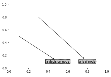
1 import matplotlib.pyplot as plt 2 3 decisionNode = dict(boxstyle="sawtooth", fc="0.8") 4 leafNode = dict(boxstyle="round4", fc="0.8") 5 arrow_args = dict(arrowstyle="<-") 6 7 def plotNode(nodeTxt, centerPt, parentPt, nodeType): 8 createPlot.ax1.annotate(nodeTxt, xy=parentPt, xycoords='axes fraction', 9 xytext=centerPt, textcoords='axes fraction', 10 va="center", ha="center", bbox=nodeType, arrowprops=arrow_args ) 11 12 def createPlot1(): 13 fig = plt.figure(1, facecolor='white') 14 fig.clf() 15 createPlot.ax1 = plt.subplot(111, frameon=False) #ticks for demo puropses 16 plotNode('a decision node', (0.5, 0.1), (0.1, 0.5), decisionNode) 17 plotNode('a leaf node', (0.8, 0.1), (0.3, 0.8), leafNode) 18 plt.show()

前面三行是定义文本框和箭头格式，decisionNode是锯齿形方框，文本框的大小是0.8，leafNode是4边环绕型，跟矩形类似，大小也是4，arrow_args是指箭头，我们在后面结果是会看到这些东西，这些数据以字典类型存储。第一个plotNode函数的功能是绘制带箭头的注解，输入参数分别是文本框的内容，文本框的中心坐标，父结点坐标和文本框的类型，这些都是通过一个createPlot.ax1.annotate函数实现的，create.ax1是一个全局变量，这个函数不多将，会用就行了。第二个函数createPlot就是生出图形，也没什么东西，函数第一行是生成图像的画框，横纵坐标最大值都是1，颜色是白色，下一个是清屏，下一个就是分图，111中第一个1是行数，第二个是列数，第三个是第几个图，这里就一个图，跟matlab中的一样，matplotlib里面的函数都是和matlab差不多。

来测试一下吧

reset -f #clear all the module and data

cd 桌面/machinelearninginaction/Ch03

/home/fangyang/桌面/machinelearninginaction/Ch03

import treePlotter import matplotlib.pyplot as plt

treePlotter.createPlot1()

2.2 构造注解树

绘制一棵完整的树需要一些技巧。我们虽然有 x 、y 坐标,但是如何放置所有的树节点却是个问题，我们必须知道有多少个叶节点,以便可以正确确定x轴的长度;我们还需要知道树有多少层，以便可以正确确定y轴的高度。这里定义了两个新函数getNumLeafs()和getTreeDepth()，以求叶节点的数目和树的层数。

参考代码：

1 def getNumLeafs(myTree): 2 numLeafs = 0 3 firstStr = myTree.keys()[0] 4 secondDict = myTree[firstStr] 5 for key in secondDict.keys(): 6 if type(secondDict[key]).__name__=='dict':#test to see if the nodes are dictonaires, if not they are leaf nodes 7 numLeafs += getNumLeafs(secondDict[key]) 8 else: numLeafs +=1 9 return numLeafs 10 11 def getTreeDepth(myTree): 12 maxDepth = 0 13 firstStr = myTree.keys()[0] 14 secondDict = myTree[firstStr] 15 for key in secondDict.keys(): 16 if type(secondDict[key]).__name__=='dict':#test to see if the nodes are dictonaires, if not they are leaf nodes 17 thisDepth = 1 + getTreeDepth(secondDict[key]) 18 else: thisDepth = 1 19 if thisDepth > maxDepth: maxDepth = thisDepth 20 return maxDepth

我们可以看到两个方法有点似曾相识，没错，我们在进行决策树分类测试时，用的跟这个几乎一样，分类测试中的isinstance函数换了一种方式去判断，递归依然在，不过是每递归依次，高度增加1，叶子数同样是检测是否为字典，不是字典则增加相应的分支。

这里还写了一个函数retrieveTree，它的作用是预先存储的树信息,避免了每次测试代码时都要从数据中创建树的麻烦

参考代码如下

1 def retrieveTree(i): 2 listOfTrees =[{'no surfacing': {0: 'no', 1: {'flippers': {0: 'no', 1: 'yes'}}}}, 3 {'no surfacing': {0: 'no', 1: {'flippers': {0: {'head': {0: 'no', 1: 'yes'}}, 1: 'no'}}}} 4 ] 5 return listOfTrees[i]

这个没什么好说的，就是把决策树的结果存在一个函数中，方便调用，跟前面的存储决策树差不多。

有了前面这些基础后，我们就可以来画树了。

参考代码如下：

1 def plotMidText(cntrPt, parentPt, txtString): 2 xMid = (parentPt[0]-cntrPt[0])/2.0 + cntrPt[0] 3 yMid = (parentPt[1]-cntrPt[1])/2.0 + cntrPt[1] 4 createPlot.ax1.text(xMid, yMid, txtString, va="center", ha="center", rotation=30) 5 6 def plotTree(myTree, parentPt, nodeTxt):#if the first key tells you what feat was split on 7 numLeafs = getNumLeafs(myTree) #this determines the x width of this tree 8 depth = getTreeDepth(myTree) 9 firstStr = myTree.keys()[0] #the text label for this node should be this 10 cntrPt = (plotTree.xOff + (1.0 + float(numLeafs))/2.0/plotTree.totalW, plotTree.yOff) 11 plotMidText(cntrPt, parentPt, nodeTxt) 12 plotNode(firstStr, cntrPt, parentPt, decisionNode) 13 secondDict = myTree[firstStr] 14 plotTree.yOff = plotTree.yOff - 1.0/plotTree.totalD 15 for key in secondDict.keys(): 16 if type(secondDict[key]).__name__=='dict':#test to see if the nodes are dictonaires, if not they are leaf nodes 17 plotTree(secondDict[key],cntrPt,str(key)) #recursion 18 else: #it's a leaf node print the leaf node 19 plotTree.xOff = plotTree.xOff + 1.0/plotTree.totalW 20 plotNode(secondDict[key], (plotTree.xOff, plotTree.yOff), cntrPt, leafNode) 21 plotMidText((plotTree.xOff, plotTree.yOff), cntrPt, str(key)) 22 plotTree.yOff = plotTree.yOff + 1.0/plotTree.totalD 23 #if you do get a dictonary you know it's a tree, and the first element will be another dict 24 25 def createPlot(inTree): 26 fig = plt.figure(1, facecolor='white') 27 fig.clf() 28 axprops = dict(xticks=[], yticks=[]) 29 createPlot.ax1 = plt.subplot(111, frameon=False, **axprops) 30 plotTree.totalW = float(getNumLeafs(inTree)) 31 plotTree.totalD = float(getTreeDepth(inTree)) 32 plotTree.xOff = -0.5/plotTree.totalW; plotTree.yOff = 1.0; 33 plotTree(inTree, (0.5,1.0), '') 34 plt.show()

第一个函数是在父子节点中填充文本信息，函数中是将父子节点的横纵坐标相加除以2，上面写得有一点点不一样，但原理是一样的，然后还是在这个中间坐标的基础上添加文本，还是用的是 createPlot.ax1这个全局变量，使用它的成员函数text来添加文本，里面是它的一些参数。

第二个函数是关键，它调用前面我们说过的函数，用树的宽度用于计算放置判断节点的位置 ,主要的计算原则是将它放在所有叶子节点的中间,而不仅仅是它子节点的中间，根据高度就可以平分坐标系了，用坐标系的最大值除以高度，就是每层的高度。这个plotTree函数也是个递归函数，每次都是调用，画出一层，知道所有的分支都不是字典后，才算画完。每次检测出是叶子，就记录下它的坐标，并写出叶子的信息和父子节点间的信息。plotTree.xOff和plotTree.yOff是用来追踪已经绘制的节点位置，以及放置下一个节点的恰当位置。

第三个函数我们之前介绍介绍过一个类似，这个函数调用了plotTree函数，最后输出树状图，这里只说两点，一点是全局变量plotTree.totalW存储树的宽度 ,全局变量plotTree.totalD存储树的深度，还有一点是plotTree.xOff和plotTree.yOff是在这个函数这里初始化的。

最后我们来测试一下

cd 桌面/machinelearninginaction/Ch03

/home/fangyang/桌面/machinelearninginaction/Ch03

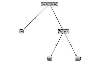
import treePlotter myTree = treePlotter.retrieveTree(0) treePlotter.createPlot(myTree)

改变标签，重新绘制图形

myTree['no surfacing'][3] = 'maybe' treePlotter.createPlot(myTree)

至此，用matplotlib画决策树到此结束。

3 使用决策树预测眼睛类型

隐形眼镜数据集是非常著名的数据集 , 它包含很多患者眼部状况的观察条件以及医生推荐的隐形眼镜类型。隐形眼镜类型包括硬材质、软材质以及不适合佩戴隐形眼镜。数据来源于UCI数据库 ,为了更容易显示数据 , 将数据存储在源代码下载路径的文本文件中。

进行测试

import trees lensesTree = trees.createTree(lenses,lensesLabels) fr = open('lenses.txt') lensesTree = trees.createTree(lenses,lensesLabels) lenses = [inst.strip().split(' ') for inst in fr.readlines()] lensesLabels = ['age' , 'prescript' , 'astigmatic','tearRate'] lensesTree = trees.createTree(lenses,lensesLabels)

lensesTree

{'tearRate': {'normal': {'astigmatic': {'no': {'age': {'pre': 'soft', 'presbyopic': {'prescript': {'hyper': 'soft', 'myope': 'no lenses'}}, 'young': 'soft'}}, 'yes': {'prescript': {'hyper': {'age': {'pre': 'no lenses', 'presbyopic': 'no lenses', 'young': 'hard'}}, 'myope': 'hard'}}}}, 'reduced': 'no lenses'}}
这样看，非常乱，看不出什么名堂，画出决策树树状图看看

treePlotter.createPlot(lensesTree)

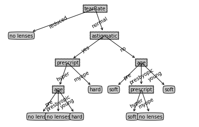
这就非常清楚了，但还是有一个问题，决策树非常好地匹配了实验数据,然而这些匹配选项可能太多了，我们将这种问题称之为过度匹配（overfitting），为了减少过度匹配问题,我们可以裁剪决策树,去掉一些不必要的叶子节点。如果叶子节点只能增加少许信息, 则可以删除该节点, 将它并人到其他叶子节点中，这个将在后面讨论吧！

结尾

这篇notebook写了两天多，接近三天，好累，希望这篇关于决策树的博客能够帮助到你，如果发现错误，还望不吝指教，谢谢！

觉得不错的，赐我金笔吧，哈哈，我需要鼓励鼓励，(^__^) 嘻嘻……

百度云盘：链接: https://pan.baidu.com/s/1eSeRQIQ 密码: 3zwm
相关阅读:
Web前端框架与类库的思考【转】
mouseover事件mouseenter事件
 11_Eclipse中演示Git版本号的创建，历史版本号的改动，创建分支，合并历史版本号和当前版本号
 实现了私聊和群聊功能的聊天工具
 有预处理命令#define声明一个常数，用以表明1年中有多少秒
 解决Office软件冲突问题
 pig载入两个不同字段个数的文件？load file with different items（f1有42列，f2有43列读到一个对象中）
游戏公司通用屏蔽字列表
 Android统计图表MPAndroidChart
HTTP状态码解析
原文地址：https://www.cnblogs.com/fydeblog/p/7159775.html

python机器学习实战（二）

1.2 划分数据集

1.3 递归构建决策树

1.4 使用决策树执行分类

1.5 决策树的存储

3 使用决策树预测眼睛类型