Neural Networks and Deep Learning（week4）Building your Deep Neural Network: Step by Step

Building your Deep Neural Network: Step by Step

你将使用下面函数来构建一个深层神经网络来实现图像分类。
使用像relu这的非线性单元来改进你的模型
构建一个多隐藏层的神经网络（有超过一个隐藏层）

^{符号说明：}

1 - Packages(导入的包)

numpy：进行科学计算的包
matplotlib ：绘图包
dnn_utils：提供一些必要功能
testCases 提供一些测试用例来评估函数的正确性
np.random.seed(1) 设置随机数种子，易于测试。

import numpy as np
import h5py
import matplotlib.pyplot as plt
from testCases_v2 import *
from dnn_utils_v2 import sigmoid, sigmoid_backward, relu, relu_backward

%matplotlib inline
plt.rcParams['figure.figsize'] = (5.0, 4.0) # 设置最大图像大小
plt.rcParams['image.interpolation'] = 'nearest'
plt.rcParams['image.cmap'] = 'gray'

%load_ext autoreload
%autoreload 2

np.random.seed(1)

保存在本地

# TODO: 保存在dnn_utils.py 
import numpy as np

def sigmoid(Z):
    """
    Implements the sigmoid activation in numpy

    Arguments:
    Z -- numpy array of any shape

    Returns:
    A -- output of sigmoid(z), same shape as Z
    cache -- returns Z as well, useful during backpropagation
    """

    A = 1/(1+np.exp(-Z))
    cache = Z

    return A, cache

def relu(Z):
    """
    Implement the RELU function.

    Arguments:
    Z -- Output of the linear layer, of any shape

    Returns:
    A -- Post-activation parameter, of the same shape as Z
    cache -- a python dictionary containing "A" ; stored for computing the backward pass efficiently
    """

    A = np.maximum(0,Z)

    assert(A.shape == Z.shape)

    cache = Z 
    return A, cache


def relu_backward(dA, cache):
    """
    Implement the backward propagation for a single RELU unit.

    Arguments:
    dA -- post-activation gradient, of any shape
    cache -- 'Z' where we store for computing backward propagation efficiently

    Returns:
    dZ -- Gradient of the cost with respect to Z
    """

    Z = cache
    dZ = np.array(dA, copy=True) # just converting dz to a correct object.

    # When z <= 0, you should set dz to 0 as well. 
    dZ[Z <= 0] = 0

    assert (dZ.shape == Z.shape)

    return dZ

def sigmoid_backward(dA, cache):
    """
    Implement the backward propagation for a single SIGMOID unit.

    Arguments:
    dA -- post-activation gradient, of any shape
    cache -- 'Z' where we store for computing backward propagation efficiently

    Returns:
    dZ -- Gradient of the cost with respect to Z
    """

    Z = cache

    s = 1/(1+np.exp(-Z))
    dZ = dA * s * (1-s)

    assert (dZ.shape == Z.shape)

    return dZ

# TODO: testCases.py
import numpy as np

def linear_forward_test_case():
    np.random.seed(1)
    """
    X = np.array([[-1.02387576, 1.12397796],
 [-1.62328545, 0.64667545],
 [-1.74314104, -0.59664964]])
    W = np.array([[ 0.74505627, 1.97611078, -1.24412333]])
    b = np.array([[1]])
    """
    A = np.random.randn(3,2)
    W = np.random.randn(1,3)
    b = np.random.randn(1,1)

    return A, W, b

def linear_activation_forward_test_case():
    """
    X = np.array([[-1.02387576, 1.12397796],
 [-1.62328545, 0.64667545],
 [-1.74314104, -0.59664964]])
    W = np.array([[ 0.74505627, 1.97611078, -1.24412333]])
    b = 5
    """
    np.random.seed(2)
    A_prev = np.random.randn(3,2)
    W = np.random.randn(1,3)
    b = np.random.randn(1,1)
    return A_prev, W, b

def L_model_forward_test_case():
    """
    X = np.array([[-1.02387576, 1.12397796],
 [-1.62328545, 0.64667545],
 [-1.74314104, -0.59664964]])
    parameters = {'W1': np.array([[ 1.62434536, -0.61175641, -0.52817175],
        [-1.07296862,  0.86540763, -2.3015387 ]]),
 'W2': np.array([[ 1.74481176, -0.7612069 ]]),
 'b1': np.array([[ 0.],
        [ 0.]]),
 'b2': np.array([[ 0.]])}
    """
    np.random.seed(1)
    X = np.random.randn(4,2)
    W1 = np.random.randn(3,4)
    b1 = np.random.randn(3,1)
    W2 = np.random.randn(1,3)
    b2 = np.random.randn(1,1)
    parameters = {"W1": W1,
                  "b1": b1,
                  "W2": W2,
                  "b2": b2}

    return X, parameters

def compute_cost_test_case():
    Y = np.asarray([[1, 1, 1]])
    aL = np.array([[.8,.9,0.4]])

    return Y, aL

def linear_backward_test_case():
    """
    z, linear_cache = (np.array([[-0.8019545 ,  3.85763489]]), (np.array([[-1.02387576,  1.12397796],
       [-1.62328545,  0.64667545],
       [-1.74314104, -0.59664964]]), np.array([[ 0.74505627,  1.97611078, -1.24412333]]), np.array([[1]]))
    """
    np.random.seed(1)
    dZ = np.random.randn(1,2)
    A = np.random.randn(3,2)
    W = np.random.randn(1,3)
    b = np.random.randn(1,1)
    linear_cache = (A, W, b)
    return dZ, linear_cache

def linear_activation_backward_test_case():
    """
    aL, linear_activation_cache = (np.array([[ 3.1980455 ,  7.85763489]]), ((np.array([[-1.02387576,  1.12397796], [-1.62328545,  0.64667545], [-1.74314104, -0.59664964]]), np.array([[ 0.74505627,  1.97611078, -1.24412333]]), 5), np.array([[ 3.1980455 ,  7.85763489]])))
    """
    np.random.seed(2)
    dA = np.random.randn(1,2)
    A = np.random.randn(3,2)
    W = np.random.randn(1,3)
    b = np.random.randn(1,1)
    Z = np.random.randn(1,2)
    linear_cache = (A, W, b)
    activation_cache = Z
    linear_activation_cache = (linear_cache, activation_cache)

    return dA, linear_activation_cache

def L_model_backward_test_case():
    """
    X = np.random.rand(3,2)
    Y = np.array([[1, 1]])
    parameters = {'W1': np.array([[ 1.78862847,  0.43650985,  0.09649747]]), 'b1': np.array([[ 0.]])}

    aL, caches = (np.array([[ 0.60298372,  0.87182628]]), [((np.array([[ 0.20445225,  0.87811744],
           [ 0.02738759,  0.67046751],
           [ 0.4173048 ,  0.55868983]]),
    np.array([[ 1.78862847,  0.43650985,  0.09649747]]),
    np.array([[ 0.]])),
   np.array([[ 0.41791293,  1.91720367]]))])
   """
    np.random.seed(3)
    AL = np.random.randn(1, 2)
    Y = np.array([[1, 0]])

    A1 = np.random.randn(4,2)
    W1 = np.random.randn(3,4)
    b1 = np.random.randn(3,1)
    Z1 = np.random.randn(3,2)
    linear_cache_activation_1 = ((A1, W1, b1), Z1)

    A2 = np.random.randn(3,2)
    W2 = np.random.randn(1,3)
    b2 = np.random.randn(1,1)
    Z2 = np.random.randn(1,2)
    linear_cache_activation_2 = ( (A2, W2, b2), Z2)

    caches = (linear_cache_activation_1, linear_cache_activation_2)

    return AL, Y, caches

def update_parameters_test_case():
    """
    parameters = {'W1': np.array([[ 1.78862847,  0.43650985,  0.09649747],
        [-1.8634927 , -0.2773882 , -0.35475898],
        [-0.08274148, -0.62700068, -0.04381817],
        [-0.47721803, -1.31386475,  0.88462238]]),
 'W2': np.array([[ 0.88131804,  1.70957306,  0.05003364, -0.40467741],
        [-0.54535995, -1.54647732,  0.98236743, -1.10106763],
        [-1.18504653, -0.2056499 ,  1.48614836,  0.23671627]]),
 'W3': np.array([[-1.02378514, -0.7129932 ,  0.62524497],
        [-0.16051336, -0.76883635, -0.23003072]]),
 'b1': np.array([[ 0.],
        [ 0.],
        [ 0.],
        [ 0.]]),
 'b2': np.array([[ 0.],
        [ 0.],
        [ 0.]]),
 'b3': np.array([[ 0.],
        [ 0.]])}
    grads = {'dW1': np.array([[ 0.63070583,  0.66482653,  0.18308507],
        [ 0.        ,  0.        ,  0.        ],
        [ 0.        ,  0.        ,  0.        ],
        [ 0.        ,  0.        ,  0.        ]]),
 'dW2': np.array([[ 1.62934255,  0.        ,  0.        ,  0.        ],
        [ 0.        ,  0.        ,  0.        ,  0.        ],
        [ 0.        ,  0.        ,  0.        ,  0.        ]]),
 'dW3': np.array([[-1.40260776,  0.        ,  0.        ]]),
 'da1': np.array([[ 0.70760786,  0.65063504],
        [ 0.17268975,  0.15878569],
        [ 0.03817582,  0.03510211]]),
 'da2': np.array([[ 0.39561478,  0.36376198],
        [ 0.7674101 ,  0.70562233],
        [ 0.0224596 ,  0.02065127],
        [-0.18165561, -0.16702967]]),
 'da3': np.array([[ 0.44888991,  0.41274769],
        [ 0.31261975,  0.28744927],
        [-0.27414557, -0.25207283]]),
 'db1': 0.75937676204411464,
 'db2': 0.86163759922811056,
 'db3': -0.84161956022334572}
    """
    np.random.seed(2)
    W1 = np.random.randn(3,4)
    b1 = np.random.randn(3,1)
    W2 = np.random.randn(1,3)
    b2 = np.random.randn(1,1)
    parameters = {"W1": W1,
                  "b1": b1,
                  "W2": W2,
                  "b2": b2}
    np.random.seed(3)
    dW1 = np.random.randn(3,4)
    db1 = np.random.randn(3,1)
    dW2 = np.random.randn(1,3)
    db2 = np.random.randn(1,1)
    grads = {"dW1": dW1,
             "db1": db1,
             "dW2": dW2,
             "db2": db2}

    return parameters, grads

2 - 任务概要

双隐藏层和 L层神经网络的 参数初始化。
实现前向传播操作（forward propagation）。计算损失函数。

完成层的 前向传播 的线性部分。(计算出
使用 relu 和 sigmod 激活函数计算结果值。
将前两个步骤组合成一个新的前向函数（线性->激活） [LINEAR->ACTIVATION]
对输出层之前的 L-1 层，做 L-1 次 的 前向传播 [LINEAR->RELU] ，L层输出层的 激活函数 为 sigmod

计算损失函数(loss fun)
实现 后向传播操作模块（在下图中用红色表示）。最后更新参数。

计算神经网络反向传播的 LINEAR 部分。
计算激活函数（Relu 或者 sigmod）的梯度。
综合前两个步骤，产生一个新的后向函数【Liner --> Activation】

更新参数

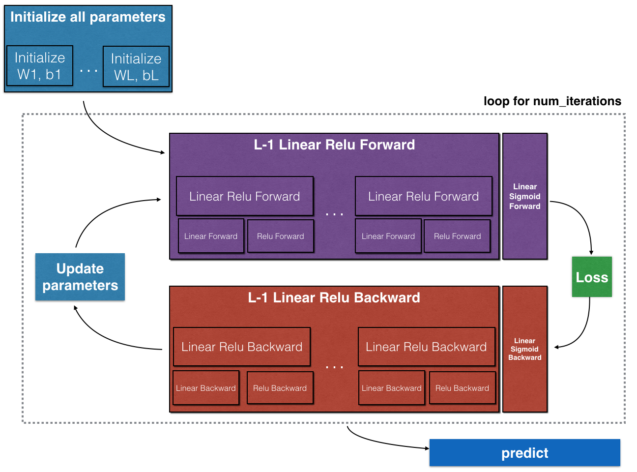
注意，前向函数和反向函数相对应。前向传播的每一步都将反向传播用的到值存储在cache。cache中值对于计算梯度非常有用。

3 - Initialization（初始化）

为你的模型编写函数初始化参数。第一个函数将用于 初始化两层模型 的参数。第二个函数用于 初始化 L层模型 的参数。

3.1 - 2-layer Neural Network (双隐藏层神经网络)

Exercise: 创建和初始化 2层神经网络的参数.

Instructions:

模型结果： LINEAR -> RELU -> LINEAR -> SIGMOID.
使用随机初始化权重矩阵。用 np.random.randn(shape)*0.01 用正确的shape。
使用 0 初始化偏差。用 np.zeros(shape)。

# GRADED FUNCTION: initialize_parameters

def initialize_parameters(n_x, n_h, n_y):
    """
    Argument:
    n_x -- size of the input layer
    n_h -- size of the hidden layer
    n_y -- size of the output layer
    
    Returns:
    parameters -- python dictionary containing your parameters:
                    W1 -- weight matrix of shape (n_h, n_x)
                    b1 -- bias vector of shape (n_h, 1)
                    W2 -- weight matrix of shape (n_y, n_h)
                    b2 -- bias vector of shape (n_y, 1)
    """
    
    np.random.seed(1)
    
    ### START CODE HERE ### (≈ 4 lines of code)
    W1 = np.random.randn(n_h, n_x)*0.01
    b1 = np.zeros((n_h, 1))
    W2 = np.random.randn(n_y, n_h)*0.01
    b2 = np.zeros((n_y, 1))
    ### END CODE HERE ###
    
    assert(W1.shape == (n_h, n_x))
    assert(b1.shape == (n_h, 1))
    assert(W2.shape == (n_y, n_h))
    assert(b2.shape == (n_y, 1))
    
    parameters = {"W1": W1,
                  "b1": b1,
                  "W2": W2,
                  "b2": b2}
    
    return parameters

parameters = initialize_parameters(3,2,1)
print("W1 = " + str(parameters["W1"]))
print("b1 = " + str(parameters["b1"]))
print("W2 = " + str(parameters["W2"]))
print("b2 = " + str(parameters["b2"]))

W1 = [[ 0.01624345 -0.00611756 -0.00528172]
 [-0.01072969  0.00865408 -0.02301539]]
b1 = [[ 0.]
 [ 0.]]
W2 = [[ 0.01744812 -0.00761207]]
b2 = [[ 0.]]

Expected output:

W1	[[ 0.01624345 -0.00611756 -0.00528172] [-0.01072969 0.00865408 -0.02301539]]
b1	[[ 0.] [ 0.]]
W2	[[ 0.01744812 -0.00761207]]
b2	[[ 0.]]

3.2 - L-layer Neural Network（L-层隐藏层神经网络）

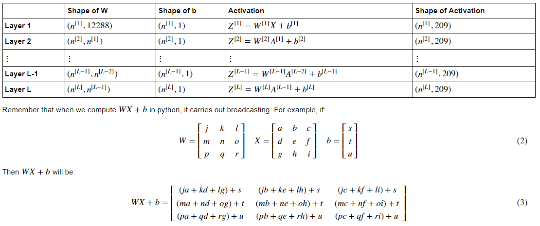
当完成 initialize_parameters_deep 时，你应该确保每个层之间的维度匹配。n^l 是 L层中单位数。如，输入X，size = (12288, 209)（有m=209个样本)：

Exercise: 实现 L层神经网络的初始化。

Instructions:

模型结构：[LINEAR -> RELU] . , 所以 L-1 层是需要用 ReLu激活函数，输出层是用 sigmod函数。
权重矩阵采用随机初始化的方式：用 np.random.randn(shape) * 0.01.
偏移矩阵仍是 0 矩阵进行初始化：用 np.zeros(shape).
我们将每层神经元数量信息进行存储，layer_dims。例如，在平面数据分类模型中 layer_dims 的值是 [2, 4, 1]：
- 其中输入层的神经元个数是2，一个隐藏层的神经元个数是 4，输出层的神经元个数是1。
- 对应 W1.shape = (4, 2), b1.shape = (4, 1)， W2.shape = (1, 4), b2.shape = (1, 1)。
下面是实现 L=1 层神经网络：

  if L == 1:
      parameters["W" + str(L)] = np.random.randn(layer_dims[1], layer_dims[0]) * 0.01
      parameters["b" + str(L)] = np.zeros((layer_dims[1], 1))

L 层神经网络实现方式（参数初始化）：

# GRADED FUNCTION: initialize_parameters_deep

def initialize_parameters_deep(layer_dims):
    """
    Arguments:
    layer_dims -- python array (list) containing the dimensions of each layer in our network
    
    Returns:
    parameters -- python dictionary containing your parameters "W1", "b1", ..., "WL", "bL":
                    Wl -- weight matrix of shape (layer_dims[l], layer_dims[l-1])
                    bl -- bias vector of shape (layer_dims[l], 1)
    """
    
    np.random.seed(3)
    parameters = {}
    L = len(layer_dims)            # number of layers in the network

    for l in range(1, L):
        ### START CODE HERE ### (≈ 2 lines of code)
        parameters['W' + str(l)] = np.random.randn(layer_dims[l], layer_dims[l - 1]) * 0.01
        parameters['b' + str(l)] = np.zeros((layer_dims[l], 1))
        ### END CODE HERE ###
        
        assert(parameters['W' + str(l)].shape == (layer_dims[l], layer_dims[l-1]))
        assert(parameters['b' + str(l)].shape == (layer_dims[l], 1))

        
    return parameters

parameters = initialize_parameters_deep([5,4,3])
print("W1 = " + str(parameters["W1"]))
print("b1 = " + str(parameters["b1"]))
print("W2 = " + str(parameters["W2"]))
print("b2 = " + str(parameters["b2"]))

Expected output:

W1	[[ 0.01788628 0.0043651 0.00096497 -0.01863493 -0.00277388] [-0.00354759 -0.00082741 -0.00627001 -0.00043818 -0.00477218] [-0.01313865 0.00884622 0.00881318 0.01709573 0.00050034] [-0.00404677 -0.0054536 -0.01546477 0.00982367 -0.01101068]]
b1	[[ 0.] [ 0.] [ 0.] [ 0.]]
W2	[[-0.01185047 -0.0020565 0.01486148 0.00236716] [-0.01023785 -0.00712993 0.00625245 -0.00160513] [-0.00768836 -0.00230031 0.00745056 0.01976111]]
b2	[[ 0.] [ 0.] [ 0.]]

4 - Forward propagation module(前向传播模型)

三个部分：

实现线性函数 (Z = np.dot(W, A) + b)
使用激励函数（Relu or Sigmod）
应用到整个模型

4.1 - Linear Forward

前向传播的过程，先计算如下的线性部分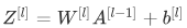：。其中，

Exercise: 建立前向传播的线性部分。

# GRADED FUNCTION: linear_forward

def linear_forward(A, W, b):
    """
    Implement the linear part of a layer's forward propagation.

    Arguments:
    A -- activations from previous layer (or input data): (size of previous layer, number of examples)
    W -- weights matrix: numpy array of shape (size of current layer, size of previous layer)
    b -- bias vector, numpy array of shape (size of the current layer, 1)

    Returns:
    Z -- the input of the activation function, also called pre-activation parameter 
    cache -- a python dictionary containing "A", "W" and "b" ; stored for computing the backward pass efficiently
    """
    
    ### START CODE HERE ### (≈ 1 line of code)
    Z = np.dot(W, A) + b
    
#     print("W: ", W.shape)
#     print("A: ", A.shape)
#     print("b: ", b.shape)
    ### END CODE HERE ###
    
    assert(Z.shape == (W.shape[0], A.shape[1]))
    cache = (A, W, b)
    
    return Z, cache

A, W, b = linear_forward_test_case()

Z, linear_cache = linear_forward(A, W, b)
print("Z = " + str(Z))

Expected output:

Z	[[ 3.26295337 -1.23429987]]

4.2 - 激活函数（相邻两层的激活实现）

你要使用的两个激励函数：

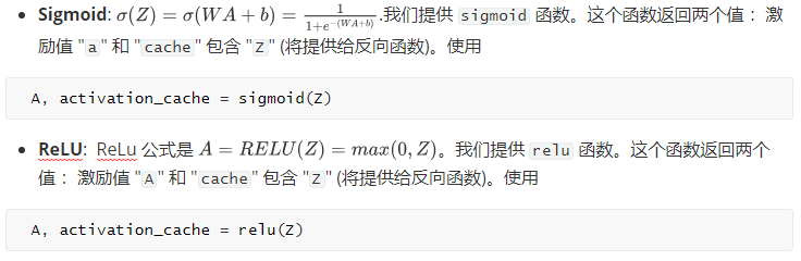
Exercise: 实现前向传播（LINEAR->ACTIVATION layer）。数学公式是：，激励函数“g”是 sigmod 或者 relu()。使用 linear_forward() 和正确的激励函数。

//预先实现的 sigmod 和 relu 函数

import numpy as np

def sigmoid(Z):
    """n
    Implements the sigmoid activation in numpy

    Arguments:
    Z -- numpy array of any shape

    Returns:
    A -- output of sigmoid(z), same shape as Z
    cache -- returns Z as well, useful during backpropagation
    """

    A = 1/(1+np.exp(-Z))
    cache = Z

    return A, cache

def relu(Z):
    """
    Implement the RELU function.

    Arguments:
    Z -- Output of the linear layer, of any shape

    Returns:
    A -- Post-activation parameter, of the same shape as Z
    cache -- a python dictionary containing "A" ; stored for computing the backward pass efficiently
    """

    A = np.maximum(0,Z)

    assert(A.shape == Z.shape)

    cache = Z 
    return A, cache

//linear_activation_forward()

# GRADED FUNCTION: linear_activation_forward

def linear_activation_forward(A_prev, W, b, activation):
    """
    Implement the forward propagation for the LINEAR->ACTIVATION layer

    Arguments:
    A_prev -- activations from previous layer (or input data): (size of previous layer, number of examples)
    W -- weights matrix: numpy array of shape (size of current layer, size of previous layer)
    b -- bias vector, numpy array of shape (size of the current layer, 1)
    activation -- the activation to be used in this layer, stored as a text string: "sigmoid" or "relu"

    Returns:
    A -- the output of the activation function, also called the post-activation value 
    cache -- a python dictionary containing "linear_cache" and "activation_cache";
             stored for computing the backward pass efficiently
    """
    
    if activation == "sigmoid":
        # Inputs: "A_prev, W, b". Outputs: "A, activation_cache".
        ### START CODE HERE ### (≈ 2 lines of code)
        Z, linear_cache = linear_forward(A_prev, W, b)   # linear_cache：A_prev, W, b
        A, activation_cache = sigmoid(Z)                 # activation_cache：Z
        ### END CODE HERE ###
    
    elif activation == "relu":
        # Inputs: "A_prev, W, b". Outputs: "A, activation_cache".
        ### START CODE HERE ### (≈ 2 lines of code)
        Z, linear_cache = linear_forward(A_prev, W, b)
        A, activation_cache = relu(Z)
        ### END CODE HERE ###
    
    assert (A.shape == (W.shape[0], A_prev.shape[1]))
    cache = (linear_cache, activation_cache)

    return A, cache

A_prev, W, b = linear_activation_forward_test_case()

A, linear_activation_cache = linear_activation_forward(A_prev, W, b, activation = "sigmoid")
print("With sigmoid: A = " + str(A))

A, linear_activation_cache = linear_activation_forward(A_prev, W, b, activation = "relu")
print("With ReLU: A = " + str(A))

Expected output:

With sigmoid: A	[[ 0.96890023 0.11013289]]
With ReLU: A	[[ 3.43896131 0. ]]

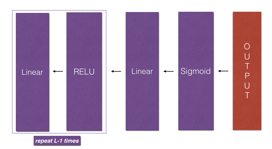
4.3 - L-Layer Model （L层模型）

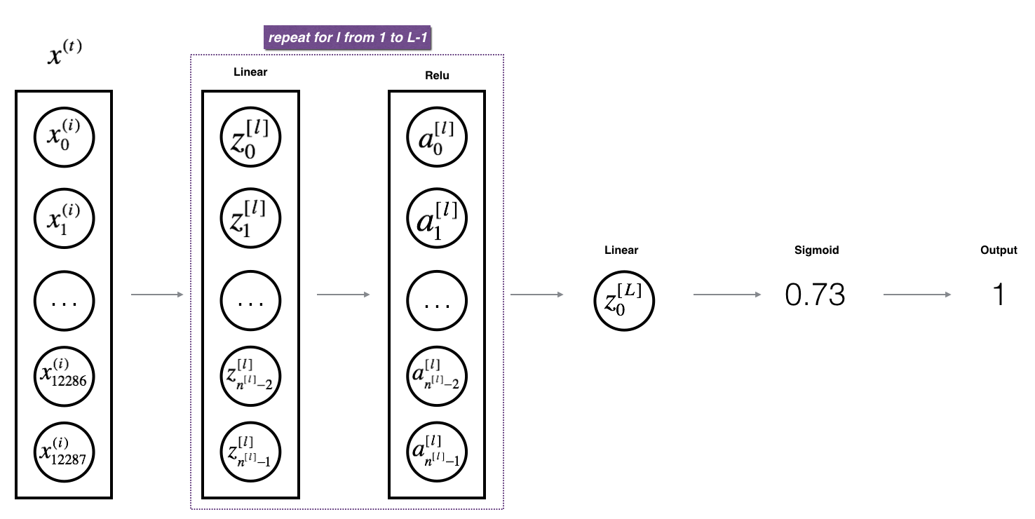
[Linear -> Relu] x (L - 1) --> Linear--> Sigmod model

Exercise: 实现以上前向传播模型

Instruction: AL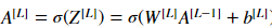：，AL有时候叫做：

Tips:

使用之前用的函数
使用循环重复【Linear --> Relu】（L-1）次
不要忘记跟踪"cache"列表中的cache。添加 c 到 list。用 list.append(c).

# GRADED FUNCTION: L_model_forward

def L_model_forward(X, parameters):
    """
    Implement forward propagation for the [LINEAR->RELU]*(L-1)->LINEAR->SIGMOID computation
    
    Arguments:
    X -- data, numpy array of shape (input size, number of examples)
    parameters -- output of initialize_parameters_deep()
    
    Returns:
    AL -- last post-activation value
    caches -- list of caches containing:
                every cache of linear_activation_forward() (there are L-1 of them, indexed from 0 to L-1)
    """

    caches = []
    A = X
    L = len(parameters) // 2                  # number of layers in the neural network
    
    # Implement [LINEAR -> RELU]*(L-1). Add "cache" to the "caches" list.
    for l in range(1, L):
        A_prev = A 
        ### START CODE HERE ### (≈ 2 lines of code)
        A, cache = linear_activation_forward(A_prev, 
                                                     parameters["W" + str(l)], 
                                                     parameters["b" + str(l)], 
                                                     activation='relu')        # cache = (A W b, Z)
        caches.append(cache)
        ### END CODE HERE ###
    
    # Implement LINEAR -> SIGMOID. Add "cache" to the "caches" list.
    ### START CODE HERE ### (≈ 2 lines of code)
    AL, cache = linear_activation_forward(A,
                                              parameters["W" + str(L)],
                                              parameters["b" + str(L)],
                                              activation="sigmoid")
    caches.append(cache)
    ### END CODE HERE ###
    
    assert(AL.shape == (1,X.shape[1]))
            
    return AL, caches

X, parameters = L_model_forward_test_case()
AL, caches = L_model_forward(X, parameters)
print("AL = " + str(AL))
print("Length of caches list = " + str(len(caches)))

AL = [[ 0.17007265 0.2524272 ]]

Length of caches list = 2

5 - Cost function(代价函数)

Exercise: 计算代价函数：

# GRADED FUNCTION: compute_cost

def compute_cost(AL, Y):
    """
    Implement the cost function defined by equation (7).

    Arguments:
    AL -- probability vector corresponding to your label predictions, shape (1, number of examples)
    Y -- true "label" vector (for example: containing 0 if non-cat, 1 if cat), shape (1, number of examples)

    Returns:
    cost -- cross-entropy cost
    """
    
    m = Y.shape[1]

    # Compute loss from aL and y.
    ### START CODE HERE ### (≈ 1 lines of code)
    cost = - (1 / m) * np.sum(np.multiply(Y, np.log(AL)) + np.multiply(1 - Y, np.log(1 - AL)))
    ### END CODE HERE ###
    
    cost = np.squeeze(cost)      # To make sure your cost's shape is what we expect (e.g. this turns [[17]] into 17).
    assert(cost.shape == ())
    
    return cost

Y, AL = compute_cost_test_case()

print("cost = " + str(compute_cost(AL, Y)))

Expected Output:

cost

0.41493159961539694

6 - Backward propagation module(反向传播模型)

反向传播用于计算损失函数相对于参数的梯度

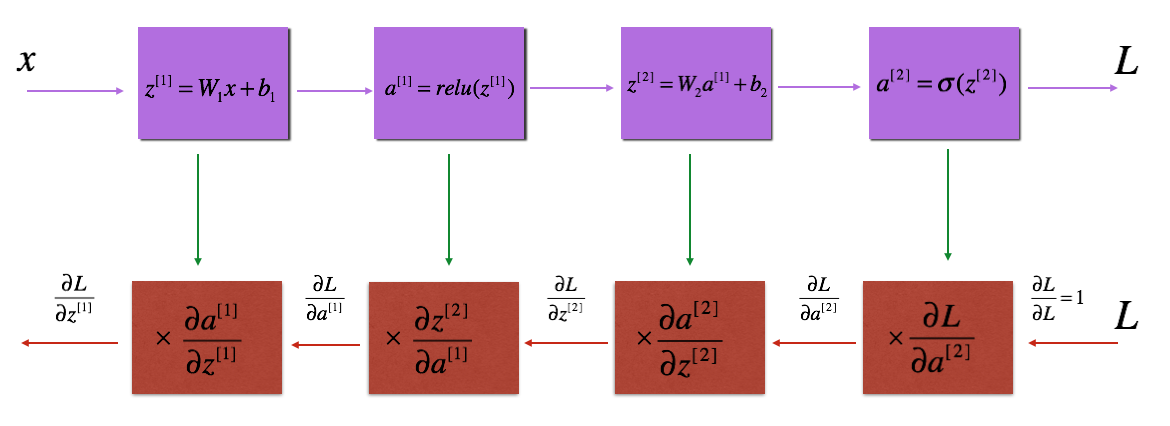
Figure3：紫色部分：前向传播；红色部分：反向传播；

建立反向传播3个步骤：

Linear backward
Linear--> Activation backward (activation 计算Relu 或者sigmod的导数)
[Linear-->Relu] x (L-1) --> Linear --> Sigmod backward (整个模型)

6.1 - Linear backward (反向传播线性部分)

对层，线性部分是：

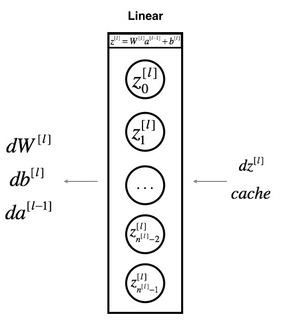
注：cache提供 tuple值 -- (A_prev, W, b）

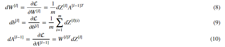
Exercise: 使用上面三个公式实现反向传播的线性部分： linear_backward().

# GRADED FUNCTION: linear_backward

def linear_backward(dZ, cache): 
    """
    Implement the linear portion of backward propagation for a single layer (layer l)

    Arguments:
    dZ -- Gradient of the cost with respect to the linear output (of current layer l)
    cache -- tuple of values (A_prev, W, b) coming from the forward propagation in the current layer

    Returns:
    dA_prev -- Gradient of the cost with respect to the activation (of the previous layer l-1), same shape as A_prev
    dW -- Gradient of the cost with respect to W (current layer l), same shape as W
    db -- Gradient of the cost with respect to b (current layer l), same shape as b
    """
    A_prev, W, b = cache    
    m = A_prev.shape[1]

    ### START CODE HERE ### (≈ 3 lines of code)
    dW = (1 / m) * np.dot(dZ, A_prev.T)
    db = (1 / m ) * np.sum(dZ, axis=1, keepdims=True)
    dA_prev = np.dot(W.T, dZ)
    ### END CODE HERE ###
    
    assert (dA_prev.shape == A_prev.shape)
    assert (dW.shape == W.shape)
    assert (db.shape == b.shape)
    
    return dA_prev, dW, db

# Set up some test inputs
dZ, linear_cache = linear_backward_test_case()

dA_prev, dW, db = linear_backward(dZ, linear_cache)
print ("dA_prev = "+ str(dA_prev))
print ("dW = " + str(dW))
print ("db = " + str(db))

Expected Output:

dA_prev	[[ 0.51822968 -0.19517421] [-0.40506361 0.15255393] [ 2.37496825 -0.89445391]]
dW	[[-0.10076895 1.40685096 1.64992505]]
db	[[ 0.50629448]]

6.2 - Linear-Activation backward

求 dz；
相邻两层的梯度实现，求(dA_prev, dW, db)

使用: linear_backward 和 用于激励的反向传播 linear_activation_backward.

为帮助你实现 linear_activation_backward, 我们提供两个反向函数：

sigmoid_backward: 实现反向传播的sigmod单元。你可以使用：

dZ = sigmoid_backward(dA, activation_cache)  # activation_cache就是Z

relu_backward: 实现反向传播的relu单元。你可以使用：

dZ = relu_backward(dA, activation_cache)

如果g(.) 是激励函数，sigmod_backward和relu_backward用来计算 。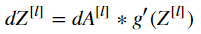

Exercise: 实现反向传播( for the LINEAR->ACTIVATION layer.)的求导部分

//预先实现的sigmoid_backward和relu_backward

def relu_backward(dA, cache):
    """
    Implement the backward propagation for a single RELU unit.

    Arguments:
    dA -- post-activation gradient, of any shape
    cache -- 'Z' where we store for computing backward propagation efficiently

    Returns:
    dZ -- Gradient of the cost with respect to Z
    """

    Z = cache
    dZ = np.array(dA, copy=True) # just converting dz to a correct object. g'(z) = 1

    # When z <= 0, you should set dz to 0 as well. 
    dZ[Z <= 0] = 0

    assert (dZ.shape == Z.shape)

    return dZ

def sigmoid_backward(dA, cache):   
    """
    Implement the backward propagation for a single SIGMOID unit.

    Arguments:
    dA -- post-activation gradient, of any shape
    cache -- 'Z' where we store for computing backward propagation efficiently

    Returns:
    dZ -- Gradient of the cost with respect to Z
    """

    Z = cache

    s = 1/(1+np.exp(-Z))
    dZ = dA * s * (1-s)     # g'(z) = s * (1 - s)

    assert (dZ.shape == Z.shape)

    return dZ

综合求 dz, dA_prev, dW, db

# GRADED FUNCTION: linear_activation_backward

def linear_activation_backward(dA, cache, activation):
    """
    Implement the backward propagation for the LINEAR->ACTIVATION layer.
    
    Arguments:
    dA -- post-activation gradient for current layer l 
    cache -- tuple of values (linear_cache, activation_cache) we store for computing backward propagation efficiently
    activation -- the activation to be used in this layer, stored as a text string: "sigmoid" or "relu"
    
    Returns:
    dA_prev -- Gradient of the cost with respect to the activation (of the previous layer l-1), same shape as A_prev
    dW -- Gradient of the cost with respect to W (current layer l), same shape as W
    db -- Gradient of the cost with respect to b (current layer l), same shape as b
    """
    linear_cache, activation_cache = cache    # A_prev W b, Z
    
    if activation == "relu":
        ### START CODE HERE ### (≈ 2 lines of code)
        dZ = relu_backward(dA, activation_cache)             # activation_cache： Z
        dA_prev, dW, db = linear_backward(dZ, linear_cache)  # linear_cache： A_prev, W, b
        ### END CODE HERE ###
        
    elif activation == "sigmoid":
        ### START CODE HERE ### (≈ 2 lines of code)
        dZ = sigmoid_backward(dA, activation_cache)
        dA_prev, dW, db = linear_backward(dZ, linear_cache)
        ### END CODE HERE ###
    
    return dA_prev, dW, db

dAL, linear_activation_cache = linear_activation_backward_test_case()

dA_prev, dW, db = linear_activation_backward(dAL, linear_activation_cache, activation = "sigmoid")
print ("sigmoid:")
print ("dA_prev = "+ str(dA_prev))
print ("dW = " + str(dW))
print ("db = " + str(db) + "
")

dA_prev, dW, db = linear_activation_backward(dAL, linear_activation_cache, activation = "relu")
print ("relu:")
print ("dA_prev = "+ str(dA_prev))
print ("dW = " + str(dW))
print ("db = " + str(db))

Expected output with sigmoid:

dA_prev	[[ 0.11017994 0.01105339] [ 0.09466817 0.00949723] [-0.05743092 -0.00576154]]
dW	[[ 0.10266786 0.09778551 -0.01968084]]
db	[[-0.05729622]]

Expected output with relu:

dA_prev	[[ 0.44090989 0. ] [ 0.37883606 0. ] [-0.2298228 0. ]]
dW	[[ 0.44513824 0.37371418 -0.10478989]]
db	[[-0.20837892]]

6.3 - L-Model Backward(L层模型)

在L_model_forward函数中每次迭代都存储了一个cache--(X, W, b, Z). 在后向传播中，你将用到这些变量来计算梯度。

在L_model_backward函数中，将遍历所有隐藏层，从L层开始。每一步中，你将使用 l 层的cache值中进行反向传播。如图：

初始化反向传播: 要通过这个网络进行反向传播，要知道输出是：。你的代码需要计算：。

使用下面公式：

dAL = - (np.divide(Y, AL) - np.divide(1 - Y, 1 - AL)) # derivative of cost with respect to AL.  -（Y / AL - (1 - Y) / (1 - AL)）

推导如下：

前向传播：

反向传播：

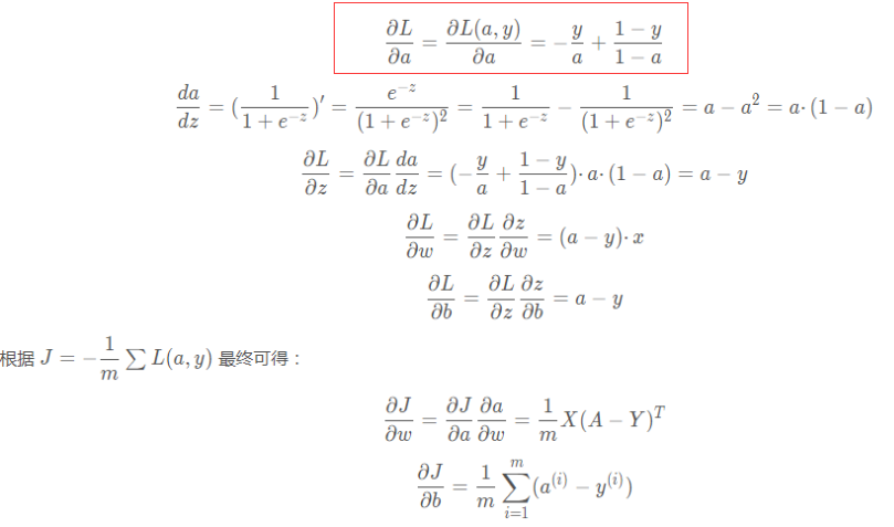
你可以用这个 dAL 来保持进行后向传播。现在，你可以使用 dAL 在 Linear-->Sigmod后向传播函数中（使用由L_model_forward函数产生的cache值）。

然后，你不得不使用一个循环来迭代每一层，使用Linear-->Relu后向传播函数。

存储每一个 dA_prev, dW, db在 grad字典中，用下列公式：$grads["dW"+str(l)] = dw^{[l])$

Exercise: 实现后向传播（[LINEAR->RELU] model）

def L_model_backward(AL, Y, caches):
    """
    Implement the backward propagation for the [LINEAR->RELU] * (L-1) -> LINEAR -> SIGMOID group

    Arguments:
    AL -- probability vector, output of the forward propagation (L_model_forward())
    Y -- true "label" vector (containing 0 if non-cat, 1 if cat)
    caches -- list of caches containing:
                every cache of linear_activation_forward() with "relu" (there are (L-1) or them, indexes from 0 to L-2)
                the cache of linear_activation_forward() with "sigmoid" (there is one, index L-1)

    Returns:
    grads -- A dictionary with the gradients
             grads["dA" + str(l)] = ... 
             grads["dW" + str(l)] = ...
             grads["db" + str(l)] = ... 
    """
    grads = {}
    L = len(caches) # the number of layers
    m = AL.shape[1]
    Y = Y.reshape(AL.shape) # after this line, Y is the same shape as AL

    # Initializing the backpropagation
    dAL = - (np.divide(Y, AL) - np.divide(1 - Y, 1 - AL))

    # Lth layer (SIGMOID -> LINEAR) gradients. Inputs: "AL, Y, caches". Outputs: "grads["dAL"], grads["dWL"], grads["dbL"]
    current_cache = caches[L-1]
    grads["dA" + str(L-1)], grads["dW" + str(L)], grads["db" + str(L)] = linear_activation_backward(dAL, current_cache, activation = "sigmoid")

    for l in reversed(range(L-1)):
        # lth layer: (RELU -> LINEAR) gradients.
        current_cache = caches[l]
        dA_prev_temp, dW_temp, db_temp = linear_activation_backward(grads["dA" + str(l + 1)], current_cache, activation = "relu")
        grads["dA" + str(l)] = dA_prev_temp
        grads["dW" + str(l + 1)] = dW_temp
        grads["db" + str(l + 1)] = db_temp

    return grads

AL, Y_assess, caches = L_model_backward_test_case()
grads = L_model_backward(AL, Y_assess, caches)
print ("dW1 = "+ str(grads["dW1"]))
print ("db1 = "+ str(grads["db1"]))
print ("dA1 = "+ str(grads["dA1"]))

Expected Output

dW1	[[ 0.41010002 0.07807203 0.13798444 0.10502167] [ 0. 0. 0. 0. ] [ 0.05283652 0.01005865 0.01777766 0.0135308 ]]
db1	[[-0.22007063] [ 0. ] [-0.02835349]]
dA1	[[ 0.12913162 -0.44014127] [-0.14175655 0.48317296] [ 0.01663708 -0.05670698]]

6.4 - Update Parameters（更新参数）

在这个任务，使用梯度下降来更新参数：

（α是学习率，在更新参数后，存储他们在参数字典中。）

Exercise: 实现 update_parameters() 来更新参数。

Instructions： 在每一个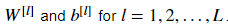，使用梯度下降来更新参数

# GRADED FUNCTION: update_parameters

def update_parameters(parameters, grads, learning_rate):
    """
    Update parameters using gradient descent
    
    Arguments:
    parameters -- python dictionary containing your parameters 
    grads -- python dictionary containing your gradients, output of L_model_backward
    
    Returns:
    parameters -- python dictionary containing your updated parameters 
                  parameters["W" + str(l)] = ... 
                  parameters["b" + str(l)] = ...
    """
    
    L = len(parameters) // 2 # number of layers in the neural network

    # Update rule for each parameter. Use a for loop.
    ### START CODE HERE ### (≈ 3 lines of code)
    for l in range(L):
        parameters["W" + str(l+1)] = parameters["W" + str(l + 1)] - grads["dW" + str(l + 1)] * learning_rate
        parameters["b" + str(l+1)] = parameters["b" + str(l + 1)] - grads["db" + str(l + 1)] * learning_rate  
    ### END CODE HERE ###
    return parameters

parameters, grads = update_parameters_test_case()
parameters = update_parameters(parameters, grads, 0.1)

print ("W1 = "+ str(parameters["W1"]))
print ("b1 = "+ str(parameters["b1"]))
print ("W2 = "+ str(parameters["W2"]))
print ("b2 = "+ str(parameters["b2"]))

Expected Output:

W1	[[-0.59562069 -0.09991781 -2.14584584 1.82662008] [-1.76569676 -0.80627147 0.51115557 -1.18258802] [-1.0535704 -0.86128581 0.68284052 2.20374577]]
b1	[[-0.04659241] [-1.28888275] [ 0.53405496]]
W2	[[-0.55569196 0.0354055 1.32964895]]
b2	[[-0.84610769]]

相关阅读:
史上最全的浏览器 CSS & JS Hack 手册
 JavaScript1.6数组新特性和JQuery的几个工具方法
 用jquery循环map
javascript强大的日期函数
 用 javascript 判断 IE 版本号
 常见排序算法基于JS的实现
 JavaScript中callee,caller,argument的理解
 apply()方法和call()方法
 虽然我们可能不想对元素应用3D变换，可我们一样可以开启3D引擎
 在移动端上加上代码，让字体变得平滑
原文地址：https://www.cnblogs.com/douzujun/p/10325980.html