▶ 使用逻辑回归来进行二分类,其中用到了梯度下降来进行数值优化
● 代码
  1 import numpy as np
  2 import matplotlib.pyplot as plt
  3 from mpl_toolkits.mplot3d import Axes3D
  4 from mpl_toolkits.mplot3d.art3d import Poly3DCollection
  5 from matplotlib.patches import Rectangle
  6
  7 dataSize = 10000
  8 trainRatio = 0.3
  9 maxTurn = 500
 10 ita = 0.1
 11 epsilon = 0.005
 12
 13 colors = [[0.5,0.25,0],[1,0,0],[0,0.5,0],[0,0,1],[1,0.5,0]] # 棕红绿蓝橙
 14 trans = 0.5
 15
 16 def dataSplit(x, y, part):
 17     return x[:part], y[:part],x[part:],y[part:]
 18
 19 def sigmod(x):                                              # 逻辑回归函数
 20     return 1.0 / (1 + np.exp(-x))
 21
 22 def function(x,para):                                       # 连续回归函数
 23     return np.sum(x * para[0]) + para[1]
 24
 25 def judge(x, para):                                         # 分类函数,由乘加部分和阈值部分组成
 26     return sigmod(function(x, para) - 0.5)
 27
 28 def createData(dim, kind, count = dataSize):                                    # 创建数据集,给定属性维度,每属性取值数,类别数,样本数
 29     np.random.seed(103)
 30     X = np.random.rand(count, dim)
 31     Y = ((3 - 2 * dim)*X[:,0] + 2 * np.sum(X[:,1:], 1) > 0.5).astype(int)
 32     #print(output)
 33     print("dim = %d, kind = %d, dataSize = %d"%(dim, kind, count))
 34     kindCount = np.zeros(kind ,dtype = int)                                     # 各类别的占比
 35     for i in range(count):
 36         kindCount[Y[i]] += 1
 37     for i in range(kind):
 38         print("kind %d -> %4f"%(i, kindCount[i]/count))
 39     return X, Y
 40
 41 def logisticRegression(dataX, dataY):                                           # 分类函数
 42     count, dim = np.shape(dataX)
 43     xE = np.concatenate((dataX, np.ones(count)[:,np.newaxis]), axis = 1)        # x 增加一列
 44     w = np.zeros(dim + 1)
 45     finishFlag = False
 46     turn = 0
 47     while finishFlag == False and turn < maxTurn:                               # 计算似然函数
 48         temp = sigmod(np.sum(xE * w, 1))
 49         error = dataY - temp
 50         grad = np.sum(xE.T * error, 1)
 51         w += ita * grad                                                         # 使用梯度下降法优化 w
 52         turn += 1
 53         #print("turn = ", turn, ", w = ", w, ", error = ", np.sum(np.abs(error)) / count)
 54         if np.sum(np.abs(error)) < count * epsilon:
 55             finishFlag = True
 56             break
 57     print("turn = ", turn, ", w = ", w)
 58     return (w[:-1],w[-1])
 59
 60 def test(dim, kind):
 61     allX, allY = createData(dim, kind)
 62     trainX, trainY, testX, testY = dataSplit(allX, allY, int(dataSize * trainRatio))    # 分离训练集
 63     para = logisticRegression(trainX, trainY)
 64
 65     myResult = [ int(judge(i, para) > 0.5) for i in testX ]
 66     errorRatio  = np.sum((np.array(myResult) != testY).astype(int)) / (dataSize * (1 - trainRatio))
 67     print("dim = %d, errorRatio = %f"%(dim, round(errorRatio,4)))
 68     if dim >= 4:                                                                        # 4维以上不画图,只输出测试错误率
 69         return
 70
 71     errorP = []                                                                         # 画图部分,测试数据集分为错误类,1 类和 0 类
 72     class1 = []
 73     class0 = []
 74     for i in range(int(dataSize * (1-trainRatio))):
 75         if int(myResult[i] > 0.5) * int(testY[i]) < 0:
 76             errorP.append(testX[i])
 77         elif myResult[i] > 0.5:
 78             class1.append(testX[i])
 79         else:
 80             class0.append(testX[i])
 81     errorP = np.array(errorP)
 82     class1 = np.array(class1)
 83     class0 = np.array(class0)
 84
 85     fig = plt.figure(figsize=(10, 8))
 86
 87     if dim == 1:
 88         plt.xlim(0.0,1.0)
 89         plt.ylim(-0.25,1.25)
 90         plt.plot([0.5, 0.5], [-0.5, 1.25], color = colors[0],label = "realBoundary")
 91         plt.plot([0, 1], [ function(i, para) for i in [0,1] ],color = colors[4], label = "myF")
 92         plt.scatter(class1, np.ones(len(class1)),color = colors[1], s = 2,label = "class1Data")
 93         plt.scatter(class0, np.zeros(len(class0)),color = colors[2], s = 2,label = "class0Data")
 94         if len(errorP) != 0:
 95             plt.scatter(errorP[:,0], errorP[:,1],color = colors[3], s = 16,label = "errorData")
 96         plt.text(0.22, 1.12, "realBoundary: 2x = 1
myF(x) = " + str(round(para[0][0],2)) + " x + " + str(round(para[1],2)) + "
 errorRatio = " + str(round(errorRatio,4)),
 97             size=15, ha="center", va="center", bbox=dict(boxstyle="round", ec=(1., 0.5, 0.5), fc=(1., 1., 1.)))
 98         R = [Rectangle((0,0),0,0, color = colors[k]) for k in range(5)]
 99         plt.legend(R, ["realBoundary", "class1Data", "class0Data", "errorData", "myF"], loc=[0.81, 0.2], ncol=1, numpoints=1, framealpha = 1)
100
101     if dim == 2:
102         plt.xlim(0.0,1.0)
103         plt.ylim(0.0,1.0)
104         plt.plot([0,1], [0.25,0.75], color = colors[0],label = "realBoundary")
105         xx = np.arange(0, 1 + 0.1, 0.1)
106         X,Y = np.meshgrid(xx, xx)
107         contour = plt.contour(X, Y, [ [ function((X[i,j],Y[i,j]), para) for j in range(11)] for i in range(11) ])
108         plt.clabel(contour, fontsize = 10,colors='k')
109         plt.scatter(class1[:,0], class1[:,1],color = colors[1], s = 2,label = "class1Data")
110         plt.scatter(class0[:,0], class0[:,1],color = colors[2], s = 2,label = "class0Data")
111         if len(errorP) != 0:
112             plt.scatter(errorP[:,0], errorP[:,1],color = colors[3], s = 8,label = "errorData")
113         plt.text(0.71, 0.92, "realBoundary: -x + 2y = 1
myF(x,y) = " + str(round(para[0][0],2)) + " x + " + str(round(para[0][1],2)) + " y + " + str(round(para[1],2)) + "
 errorRatio = " + str(round(errorRatio,4)),
114             size = 15, ha="center", va="center", bbox=dict(boxstyle="round", ec=(1., 0.5, 0.5), fc=(1., 1., 1.)))
115         R = [Rectangle((0,0),0,0, color = colors[k]) for k in range(4)]
116         plt.legend(R, ["realBoundary", "class1Data", "class0Data", "errorData"], loc=[0.81, 0.2], ncol=1, numpoints=1, framealpha = 1)
117
118     if dim == 3:
119         ax = Axes3D(fig)
120         ax.set_xlim3d(0.0, 1.0)
121         ax.set_ylim3d(0.0, 1.0)
122         ax.set_zlim3d(0.0, 1.0)
123         ax.set_xlabel('X', fontdict={'size': 15, 'color': 'k'})
124         ax.set_ylabel('Y', fontdict={'size': 15, 'color': 'k'})
125         ax.set_zlabel('W', fontdict={'size': 15, 'color': 'k'})
126         v = [(0, 0, 0.25), (0, 0.25, 0), (0.5, 1, 0), (1, 1, 0.75), (1, 0.75, 1), (0.5, 0, 1)]
127         f = [[0,1,2,3,4,5]]
128         poly3d = [[v[i] for i in j] for j in f]
129         ax.add_collection3d(Poly3DCollection(poly3d, edgecolor = 'k', facecolors = colors[0]+[trans], linewidths=1))
130         ax.scatter(class1[:,0], class1[:,1],class1[:,2], color = colors[1], s = 2, label = "class1")
131         ax.scatter(class0[:,0], class0[:,1],class0[:,2], color = colors[2], s = 2, label = "class0")
132         if len(errorP) != 0:
133             ax.scatter(errorP[:,0], errorP[:,1],errorP[:,2], color = colors[3], s = 8, label = "errorData")
134         ax.text3D(0.75, 0.85, 1.15, "realBoundary: -3x + 2y +2z = 1
myF(x,y,z) = " + str(round(para[0][0],2)) + " x + " +
135             str(round(para[0][1],2)) + " y + " + str(round(para[0][2],2)) + " z + " + str(round(para[1],2)) + "
 errorRatio = " + str(round(errorRatio,4)),
136             size = 12, ha="center", va="center", bbox=dict(boxstyle="round", ec=(1, 0.5, 0.5), fc=(1, 1, 1)))
137         R = [Rectangle((0,0),0,0, color = colors[k]) for k in range(4)]
138         plt.legend(R, ["realBoundary", "class1Data", "class0Data", "errorData"], loc=[0.83, 0.1], ncol=1, numpoints=1, framealpha = 1)
139
140     fig.savefig("R:\dim" + str(dim) + ".png")
141     plt.close()
142
143 if __name__=='__main__':
144     test(1, 2)
145     test(2, 2)
146     test(3, 2)
147     test(4, 2)
148
● 输出结果
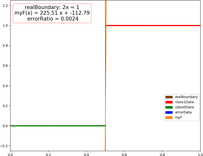
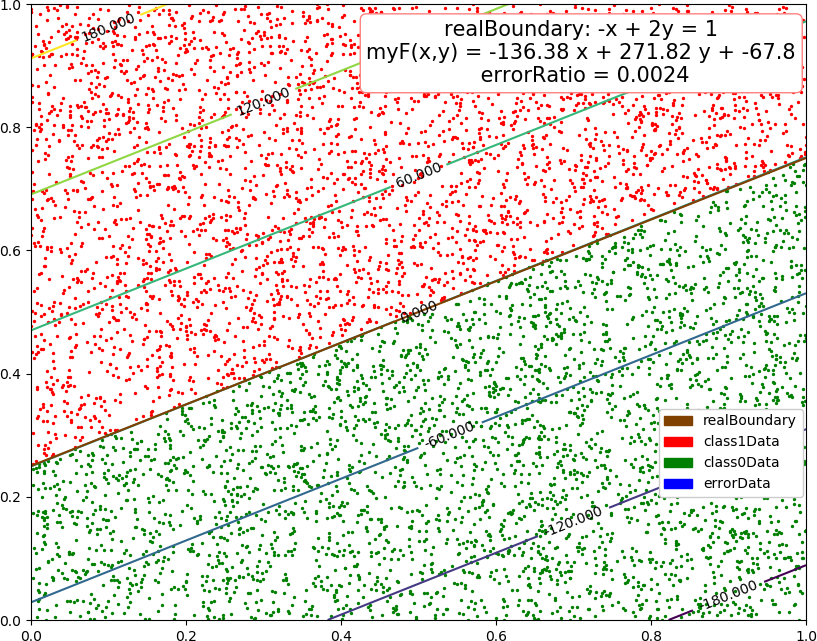
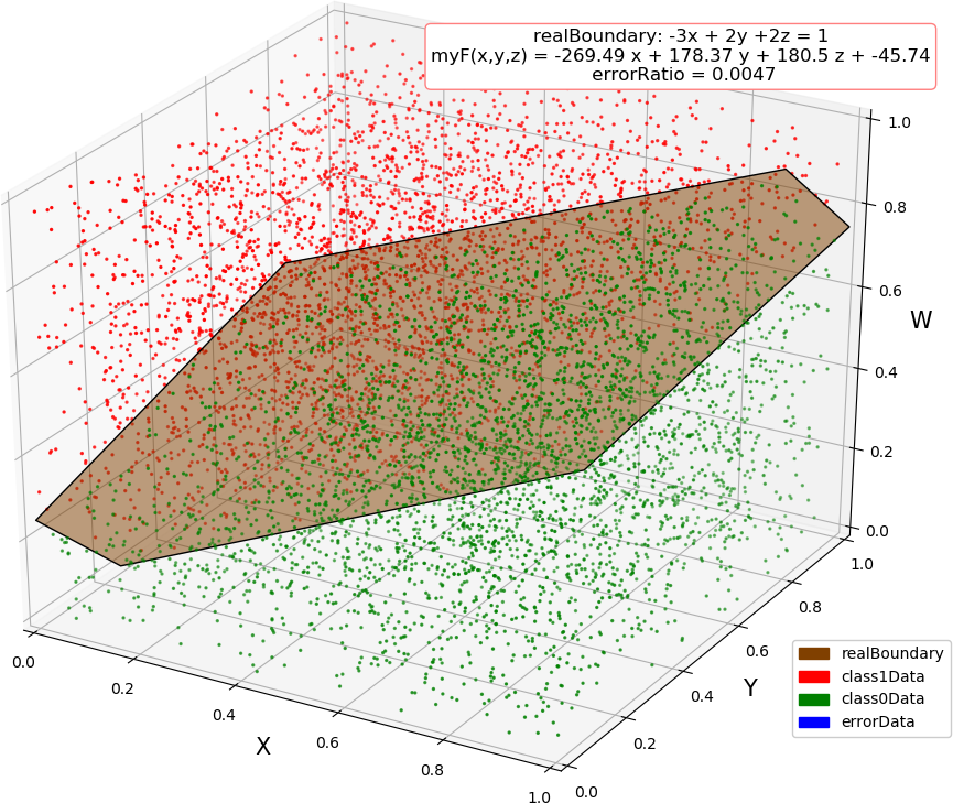
dim = 1, kind = 2, dataSize = 10000
kind 0 -> 0.491000
kind 1 -> 0.509000
turn =  500 , w =  [ 225.51391655 -112.78995202]
dim = 1, errorRatio = 0.002400
dim = 2, kind = 2, dataSize = 10000
kind 0 -> 0.504000
kind 1 -> 0.496000
turn =  500 , w =  [-136.38367654  271.82263114  -67.80046401]
dim = 2, errorRatio = 0.002400
dim = 3, kind = 2, dataSize = 10000
kind 0 -> 0.501800
kind 1 -> 0.498200
turn =  76 , w =  [-269.48732449  178.37270183  180.50103751  -45.74231996]
dim = 3, errorRatio = 0.004700
dim = 4, kind = 2, dataSize = 10000
kind 0 -> 0.503100
kind 1 -> 0.496900
turn =  74 , w =  [-335.00400878  133.17805105  132.39352473  132.93672898  -31.98460298]
dim = 4, errorRatio = 0.002100
● 画图