机器学习-线性模型（线性回归与逻辑回归）

date: 2019-03-31 00:58

一、线性模型（linear model）

线性模型试图学习一个通过属性关系的线性组合来进行预测的函数。

表达式如下：

[f(x)={w_{1}}{x_{1}}+{w_{2}}{x_{2}}+...+{w_{d}}{x_{d}}+b ]

向量形式为：

[f(x)=mathbf{w}^{T}mathbf{x}+b ]

其中 $$mathbf{w}=({w_{1};w_{2};}...;w_{d};)$$
当 $$mathbf{w}$$ 和 b 学得后，模型就得以确定。

二、线性回归（linear regression）

线性回归试图学得一个线性模型，以尽可能准确地预测实值输出标记。

简单的一元线性回归（输入属性的数目只有一个）：

[f({x_{i}})=w{x_{i}}+b ]

那么如何确定 w 和 b 呢？

试图让 均方误差 最小化：

[(w^{*},b^{*})=underset{(w,b)}{argmin}sum_{i=1}^{m}{(f(x_i)-y_i)^2}=underset{(w,b)}{argmin}sum_{i=1}^{m}{(y_i-wx_i-b)^2} ]

其中 $$w^{*},b{*}$$表示 w 和 b 的解。

基于均方误差最小化来进行模型求解的方法称为 最小二乘法（least square method）

求解 w 和 b 使$$E_{(w,b)}=sum_{i=1}^{{m}{(y_i-wx_i-b)}2}$$最小化的过程，称为线性模型的 最小二乘“参数估计”（parameter estimation）。

这里$$E_{(w,b)}$$是关于 w 和 b 的凸函数，当它关于 w 和 b 的导数均为零时，得到 w 和 b 的最优解。

多元线性回归（multivariate linear regression）

对于数据集 D，样本有 d 个属性描述，多元线性回归试图学得：

[f(mathbf{x}_i)=mathbf{w}^Tmathbf{x}_i+b ]

使得$$f(mathbf{w}_i)simeq y_i$$。

同样，使用最小二乘法来对 w 和 b 进行估计。 为了便于讨论，把 w 和 b 吸收入向量形式$$hat{mathbf{w}}=(mathbf{w};b)$$，数据集 D 表示为一个 m*(d+1) 大小的矩阵 $$mathbf{X}$$，其中每一行对应于一个示例，每行前 d 个元素代表示例的 d 个属性值，最后一个元素恒置为1，即：

[mathbf{X}=egin{pmatrix} x_{11} & x_{12} & cdots & x_{1d} & 1\ x_{21} & x_{22} & cdots & x_{2d} & 1\ vdots & vdots & ddots & vdots & vdots\ x_{m1} & x_{m2} & cdots & x_{md} & 1 end{pmatrix}=egin{pmatrix} mathbf{x}_1^T & 1 \ mathbf{x}_2^T & 1 \ vdots & vdots \ mathbf{x}_m^T & 1 end{pmatrix} ]

再把标记写成向量形式$$mathbf{y}=(y_1;y_2;...;y_m)$$，则有：

[hat{mathbf{w}}^*=underset{hat{mathbf{w}}}{argmin}(mathbf{y}-mathbf{X}hat{mathbf{w}})^Tunderset{hat{mathbf{w}}}{argmin}(mathbf{y}-mathbf{X}hat{mathbf{w}}) ]

令$$E_{hat{mathbf{w}}}=(mathbf{y}-mathbf{X}hat{mathbf{w}})^T(mathbf{y}-mathbf{X}hat{mathbf{w}})$$，对$$hat{mathbf{w}}$$求导得：

[frac{partial E_{hat{mathbf{w}}}}{partial hat{mathbf{w}}}=2mathbf{X}^T(mathbf{X}hat{mathbf{w}}-mathbf{y}) ]

令上式为零可得最优解的闭式解。

下面做一个简单的讨论，当$$mathbf{X}^Tmathbf{X}$$为满秩矩阵或正定矩阵时，令上式为零可得：

[hat{mathbf{w}}=(mathbf{X}^Tmathbf{X})^{-1}mathbf{X}^Tmathbf{y} ]

其中$$(mathbf{X}^Tmathbf{X}){-1}$$是矩阵$$(mathbf{X}^Tmathbf{X})$$的逆矩阵。令$$hat{mathbf{x}}=(mathbf{x_i},1)$$，则最终学得的多元线性模型为：

[f(mathbf{hat{x}})=hat{mathbf{x}}^T(mathbf{X}mathbf{X}^T)^{-1}mathbf{X}^Tmathbf{y} ]

三、逻辑回归（logistic regression）

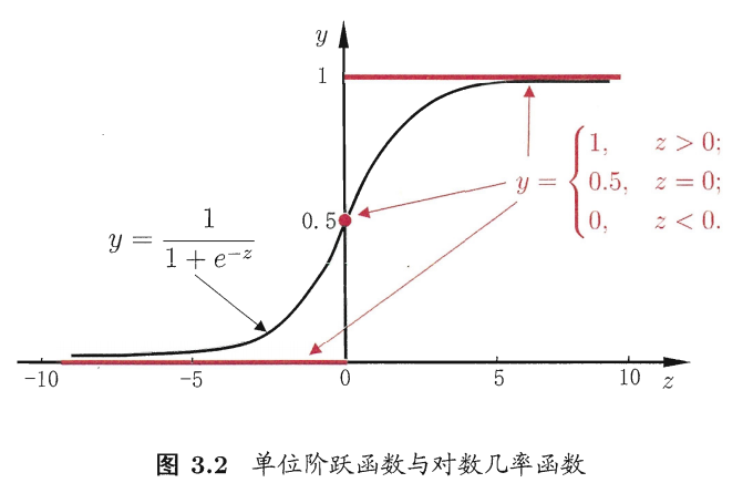
用线性模型为预测结果去逼近真实标记的几率函数，称为对数几率函数（逻辑回归）。

为了使线性模型可以做分类任务，需要找一个单调可微函数将分类任务的真实标记 y 与线性回归模型的预测值联系起来。

这里很容易想到的是“单位阶跃函数”（unit-step function），但是该函数不连续。

Sgmoid 函数：形似 S 的函数，对率函数是它最重要的代表。
对数几率函数（logistic function）：

[y=frac{1}{1+e^{-z}} ]

如图所示：

将线性模型的预测值带入到对数几率函数中，用 g(z) 表示对数几率函数的值，可得：

[g(z)=frac{1}{1+e^{-(mathbf{w}^Tmathbf{x}+b)}} ]

此时，g(z)的值不是预测结果值，而是一个值预测为正例的概率，预测为负例的概率就是 1-g(z).
函数形式表达：

[p(y=0|mathbf{x})=g(z)\ p(y=1|mathbf(x))=1-g(z) ]

到这里，逻辑回归的原理基本就清楚了，判别函数就是 g(z).

四、推倒过程

见南瓜书：南瓜书PumpkinBook - 第3章 线性模型

五、线性回归和逻辑回归的算法实现

手写代码实现算法便于理解算法本质：

• 线性回归
• 逻辑回归

六、sklearn库中线性回归的使用方法

[f(x)=mathbf{w}^{T}mathbf{x}+b ]

在整个模块中，定义$$mathbf{w}=({w_{1};w_{2};}...;w_{d};)$$为 coef_，定义 b 为 intercept_。
LinearRegression拟合一个带有系数$$mathbf{w}=({w_{1};w_{2};}...;w_{d};)$$的线性模型，使得数据集的实际观测数据和预测值之间的均方误差最小，公式如下：

[min_{w} {|| X w - y||_2}^2 ]

LinearRegression会调用fit()函数来拟合$$mathbf{X}$$和$$mathbf{y}$$，并将线性模型的系数保存在成员变量coef_中。

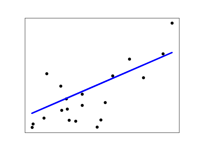
案例：

import matplotlib.pyplot as plt
import numpy as np
from sklearn import datasets, linear_model
from sklearn.metrics import mean_squared_error, r2_score

# Load the diabetes dataset
diabetes = datasets.load_diabetes()


# Use only one feature
diabetes_X = diabetes.data[:, np.newaxis, 2]

# Split the data into training/testing sets
diabetes_X_train = diabetes_X[:-20]
diabetes_X_test = diabetes_X[-20:]

# Split the targets into training/testing sets
diabetes_y_train = diabetes.target[:-20]
diabetes_y_test = diabetes.target[-20:]

# Create linear regression object
regr = linear_model.LinearRegression()

# Train the model using the training sets
regr.fit(diabetes_X_train, diabetes_y_train)

# Make predictions using the testing set
diabetes_y_pred = regr.predict(diabetes_X_test)

# The coefficients
print('Coefficients: 
', regr.coef_)
# The mean squared error
print("Mean squared error: %.2f"
      % mean_squared_error(diabetes_y_test, diabetes_y_pred))
# Explained variance score: 1 is perfect prediction
print('Variance score: %.2f' % r2_score(diabetes_y_test, diabetes_y_pred))

# Plot outputs
plt.scatter(diabetes_X_test, diabetes_y_test,  color='black')
plt.plot(diabetes_X_test, diabetes_y_pred, color='blue', linewidth=3)

plt.xticks(())
plt.yticks(())

plt.show()

输出：

Coefficients: 
 [938.23786125]
Mean squared error: 2548.07
Variance score: 0.47

七、sklearn库中的逻辑回归的使用方法

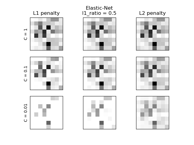
scikit-learn 中 logistic 回归在 LogisticRegression 类中实现了二分类（binary）、一对多分类（one-vs-rest）及多项式 logistic 回归，并带有可选的 L1 和 L2 正则化。

案例：

import numpy as np
import matplotlib.pyplot as plt

from sklearn.linear_model import LogisticRegression
from sklearn import datasets
from sklearn.preprocessing import StandardScaler

digits = datasets.load_digits()

X, y = digits.data, digits.target
X = StandardScaler().fit_transform(X)

y = (y > 4).astype(np.int)

# Set regularization parameter
for i, C in enumerate((1, 0.1, 0.01)):
    # turn down tolerance for short training time
    clf_l1_LR = LogisticRegression(C=C, penalty='l1', tol=0.01, solver='saga')
    clf_l2_LR = LogisticRegression(C=C, penalty='l2', tol=0.01, solver='saga')
    clf_l1_LR.fit(X, y)
    clf_l2_LR.fit(X, y)

    coef_l1_LR = clf_l1_LR.coef_.ravel()
    coef_l2_LR = clf_l2_LR.coef_.ravel()

    # coef_l1_LR contains zeros due to the
    # L1 sparsity inducing norm

    sparsity_l1_LR = np.mean(coef_l1_LR == 0) * 100
    sparsity_l2_LR = np.mean(coef_l2_LR == 0) * 100

    print("C=%.2f" % C)
    print("Sparsity with L1 penalty: %.2f%%" % sparsity_l1_LR)
    print("score with L1 penalty: %.4f" % clf_l1_LR.score(X, y))
    print("Sparsity with L2 penalty: %.2f%%" % sparsity_l2_LR)
    print("score with L2 penalty: %.4f" % clf_l2_LR.score(X, y))

    l1_plot = plt.subplot(3, 2, 2 * i + 1)
    l2_plot = plt.subplot(3, 2, 2 * (i + 1))
    if i == 0:
        l1_plot.set_title("L1 penalty")
        l2_plot.set_title("L2 penalty")

    l1_plot.imshow(np.abs(coef_l1_LR.reshape(8, 8)), interpolation='nearest',
                   cmap='binary', vmax=1, vmin=0)
    l2_plot.imshow(np.abs(coef_l2_LR.reshape(8, 8)), interpolation='nearest',
                   cmap='binary', vmax=1, vmin=0)
    plt.text(-8, 3, "C = %.2f" % C)

    l1_plot.set_xticks(())
    l1_plot.set_yticks(())
    l2_plot.set_xticks(())
    l2_plot.set_yticks(())

plt.show()

输出：

C=1.00
Sparsity with L1 penalty: 6.25%
score with L1 penalty: 0.9093
Sparsity with L2 penalty: 4.69%
score with L2 penalty: 0.9048
C=0.10
Sparsity with L1 penalty: 29.69%
score with L1 penalty: 0.9009
Sparsity with L2 penalty: 4.69%
score with L2 penalty: 0.9032
C=0.01
Sparsity with L1 penalty: 84.38%
score with L1 penalty: 0.8620
Sparsity with L2 penalty: 4.69%
score with L2 penalty: 0.8887

LogisticRegressionCV 对 logistic 回归 的实现内置了交叉验证（cross-validation），可以找出最优的参数 C 。

参数解读：
关于参数说明，网上和官网都有很多，这里我将一个通俗易懂的直接搬过来：

参数名称	注释	备注
penalty	用于选择正则化项。参数值为'l1'时，表示正则化项为 L1 正则化参数值为’l2’时，表示正则化项为L2正则化。	新目标函数二目标函数+正则化项正则化项是防止模型过拟合的最为常用的手段之一。
dual	选择目标函数为原始形式还是其对偶形式。	何为对偶函数？将原始函数等价转换为一个新函数，这个新函数我们称为对偶函数。对偶函数比原始函数更易于优化。
Tol	优化算法停止的条件。	一般优化算法都是迭代算法，举个例子，比如牛顿法，假设我们现在要最小化一个函数，每迭代一次，更新一次变量值，函数的值都要减少一点，就这样一直迭代下去。那么应该什么时候停止呢，比如我们设 tol=0.001，就是当迭代前后的函数差值<=0.001时就停止。
C	用来控制正则化项的强弱。C越小，正则化越强。	可以简单把C理解成正则化项的系数的倒数。
fit_intercept	用来选择逻辑回归模型中是否含有b.	b 即线性模型的常数项。如果不含有 b，即等价于 b=0
intercept_scaling		在西瓜书算法中会有一个步骤，令x= (x,1)，但是在具体的代码实现上是:x=(x,intercept_scaling) ((x，1)意思就是在向量x后加一个数值1，形成一个新的向量)
class_weight	设置每个类别的权重。	在西瓜书3.先自己计算好，然后再赋值。也可以设置 class_ weight 为 balanced,即让程序自动根据数据集计算每个类别对应的权重值。
random_state	随机数种子。	在程序中.有很名变量的初始值都是随机产生的值，那么这个种子就是控制产生什么值。比如，为种子值为20，那么每次随机产生的值都是20这个种子对应的值。而且很多时候，数据集中每个样的顺序需要进行打乱，那么这个种子就是控制打乱后的顺序的。
solver	选择使用哪个优化算法进行优化。	对于一个目标函数，我们可以有很多优化算法供我们进行选择，因为不同的优化算法所擅长解决的问题是不同。
max_iter	优化算法的迭代次数	前面参数中介绍了，我们可以用 tol 参数来控制优化算法是否停止。还有就是，我们也可以用迭代次数来控制停止与否。
multi_class	用于选择多分类的策略	由西瓜书3.5可知，用二分类器去构造出一个多分类器，有很多可供选择的策略，比如 ovo,ovr,mvm。注意，从数学理论上来讲，我们可以构造出一个多分类函数，但是在实践过程中，我们并不这样做，更一般的做法是用多个二分类器构造出一个多分类器。还有 softmax 同归带略。
verbose	主要用来控制是否print训练过程
warm_start	是否热启动	什么叫热启动呢?一般而言，当我们定义一个机器学习模型时，就是定义其参数变量，所以要在一开始阶段，对变量进行随机地初始化。但是热启动的意思是，我们不在随机地初始化而是把之前训练好的参数值赋值给变量进行初始化。
n_jobs	用cpu的几个核来跑程序

---

参考：

• 《机器学习》周志华
• Scikit-learn官方文档
• Scikit-learn 0.19.x 中文文档
• Sklearn-LogisticRegression逻辑回归
• LogisticRegression参数