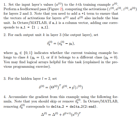
The goal of backpropagation is to compute the partial derivatives ∂C/∂w and ∂C/∂b of the cost function C with respect to any weight ww or bias b in the network.
we use the quadratic cost function

two assumptions :
1: The first assumption we need is that the cost function can be written as an average
 (case for the quadratic cost function)
The reason we need this assumption is because what backpropagation actually lets us do is compute the partial derivatives
∂Cx/∂w and ∂Cx/∂b for a single training example. We then recover ∂C/∂w and ∂C/∂b by averaging over training examples. In
fact, with this assumption in mind, we'll suppose the training example x has been fixed, and drop the x subscript, writing the
cost Cx as C. We'll eventually put the x back in, but for now it's a notational nuisance that is better left implicit.
2: The cost function can be written as a function of the outputs from the neural network
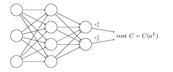
the Hadamard product
(s⊙t)j=sjtj(s⊙t)j=sjtj

The four fundamental equations behind backpropagation
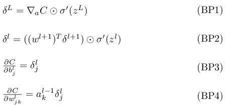
BP1
 :the error in the jth neuron in the lth layer

You might wonder why the demon is changing the weighted input zlj. Surely it'd be more natural to imagine the demon changing
the output activation alj, with the result that we'd be using ∂C/∂alj as our measure of error. In fact, if you do this things work out quite
similarly to the discussion below. But it turns out to make the presentation of backpropagation a little more algebraically complicated.
So we'll stick with δlj=∂C/∂zlj as our measure of error.
An equation for the error in the output layer, δL: The components of δL are given by

it's easy to rewrite the equation in a matrix-based form, as


BP2


BP3

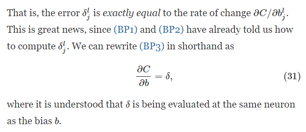
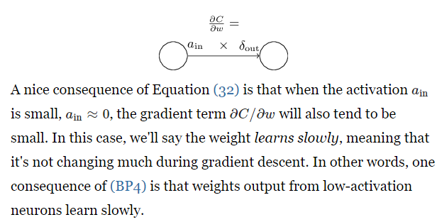
BP4


The backpropagation algorithm
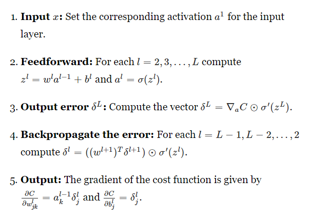

Of course, to implement stochastic gradient descent in practice you also need an outer loop generating mini-batches
of training examples, and an outer loop stepping through multiple epochs of training. I've omitted those for simplicity.
reference: http://neuralnetworksanddeeplearning.com/chap2.html

