About the Mean Shift

Mean Shift算法，一般是指一个迭代的过程。即先算出当前点的偏移均值,移动该点到其偏移均值，然后以此为新的起始点,继续移动，直到满足一定的条件结束。

meanshift可以被用来做目标跟踪和图像分割。

参考《Mean Shift：A Robust Approach Toward Feature Space Analysis》

        公式就不写了。meanshift其实原理挺简单的，就是随便找个种子点，然后开始在该种子点邻域内寻找其目标点的密度中心，那么种子点到密度中心点的向量方向就是密度上升方向了，更新密度中心点为种子点，迭代，直到到达截止条件（opencv里的meanshift把截止条件定为迭代次数和截止精度，当然这两者可以随意组合）。

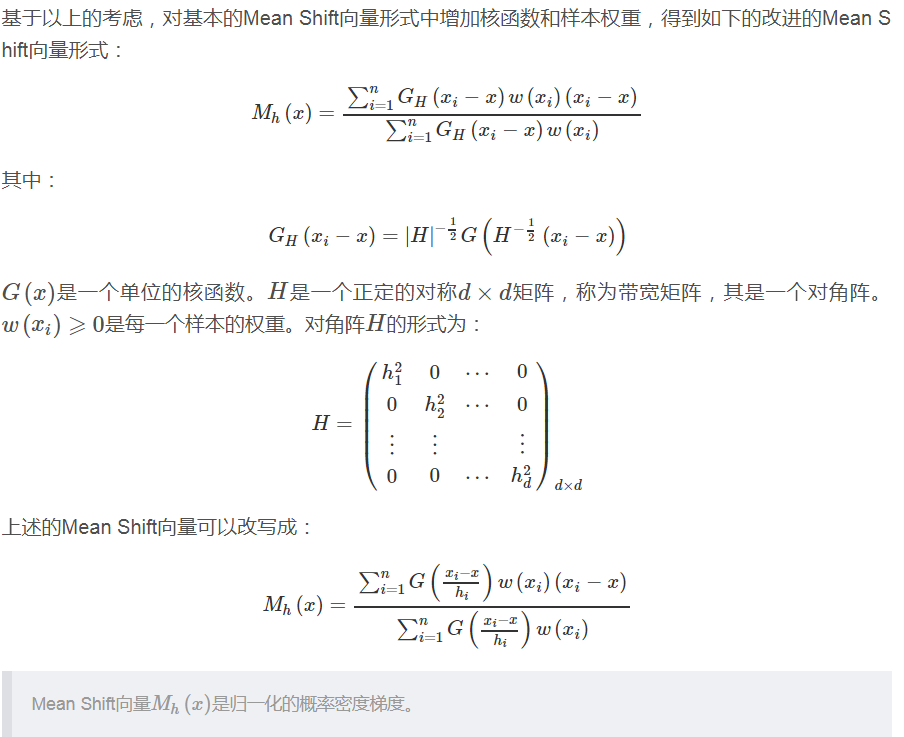
        改进的meanshift使用了核函数（区别种子点附近和远处点的权重）和权重系数（区别不同样本的权重），但基本原理还是一样的。

        这篇论文很长，在实现该方法的同时，同时系统地证明了meanshift算法是沿着最大密度梯度方向搜索的，并且随着多次迭代，种子点趋于稳定。

        其实在上面讲述的时候去掉了一个背景，就是所有样本都采样自概率密度函数，但这并不影响我们理解其原理。

       

        通过分析meanshift的原理，其目的就是寻找局部最优点，这样很容易联想到它在图像分割或聚类上的应用。

        对于图像处理方面的应用，其样本可认为是（x，y），x值二维坐标，y是颜色空间（p维，maybe  1or3），那么总维数是p+2。

        meanshift也可用作图像平滑，但是对每一个像素点操作用迭代截止值代替，算法复杂度肯定很高了。

        用meanshift算法做目标跟踪时，先预先取一个目标矩形框，在目标移动的时候，就会迭代更新密度中心点到当前目标的密度中心，这样只是一个固定的矩形框的局部范围搜索，算法复杂度肯定可以接受，实时性就不错了。但是通过分析发现用meanshift做跟踪的话，目标突然消失又突然出现，这个算法就凉凉了，所以换句话说，目标必须连续移动。

　　关于用meanshift做图像分割，后面详细介绍：

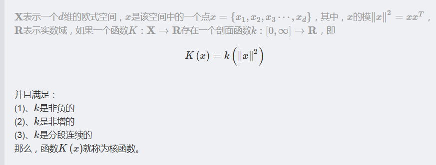
一、Mean Shift算法概述

Mean Shift算法又称均值漂移算法，Mean Shift的概念最早是由Fukunage在1975年提出的，在后来又由Yzong Cheng对其进行扩充，主要提出了两点改进：

定义了核函数；

增加了权重系数。

核函数的定义使得偏移向量的贡献随着样本与被偏移点的距离的不同而不同。

权重系数使得不同样本的权重不同。Mean Shift算法在聚类，图像平滑，分割以及视频跟踪等方面有广泛的应用。

二、算法原理

2.1、核函数

核函数性质参见：http://www.cnblogs.com/liqizhou/archive/2012/05/11/2495788.html

在Mean Shift算法中引入核函数的目的是：随着样本与被偏移点距离的不同，其偏移量对均值偏移向量的贡献也不同。核函数是机器学习中常用的一种方式，核函数的定义如下：

常用的核函数有高斯核函数。高斯核函数如下所示：

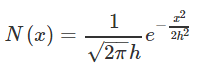
其中，h称为带宽(bandwidth)，不同带宽的核函数如下图所示：

附上画出上图的python代码：

import matplotlib.pyplot as plt
import math

def cal_Gaussian(x, h=1):
    molecule = x * x
    denominator = 2 * h * h
    left = 1 / (math.sqrt(2 * math.pi) * h)
    return left * math.exp(-molecule / denominator)

x = []

for i in range(-40,40):
    x.append(i * 0.5);

score_1 = []
score_2 = []
score_3 = []
score_4 = []

for i in x:
    score_1.append(cal_Gaussian(i,1))
    score_2.append(cal_Gaussian(i,2))
    score_3.append(cal_Gaussian(i,3))
    score_4.append(cal_Gaussian(i,4))

plt.plot(x, score_1, 'b--', label="h=1")
plt.plot(x, score_2, 'k--', label="h=2")
plt.plot(x, score_3, 'g--', label="h=3")
plt.plot(x, score_4, 'r--', label="h=4")

plt.legend(loc="upper right")
plt.xlabel("x")
plt.ylabel("N")
plt.show()

2.2、Mean Shift算法的核心思想

2.2.1、基本原理

对于Mean Shift算法，是一个迭代的过程，即先算出当前点的偏移均值，将该点移动到此偏移均值，然后以此为新的起始点，继续移动，直到满足最终的条件。

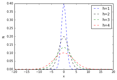
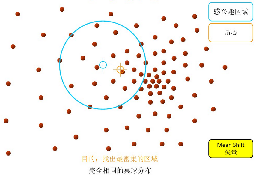
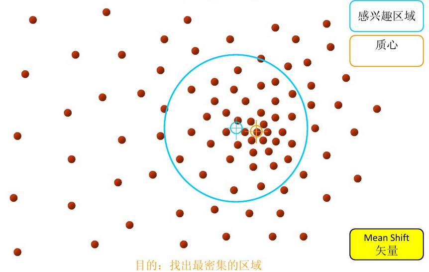
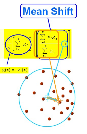
以上是官方的说法，即书上的定义，个人理解就是，在d维空间中，任选一个点，然后以这个点为圆心，h为半径做一个高维球，因为有d维，d可能大于2，所以是高维球。落在这个球内的所有点和圆心都会产生一个向量，向量是以圆心为起点落在球内的点位终点。然后把这些向量都相加。相加的结果就是Meanshift向量。

步骤1：在指定的区域内计算偏移均值(下图中黄色的圈)

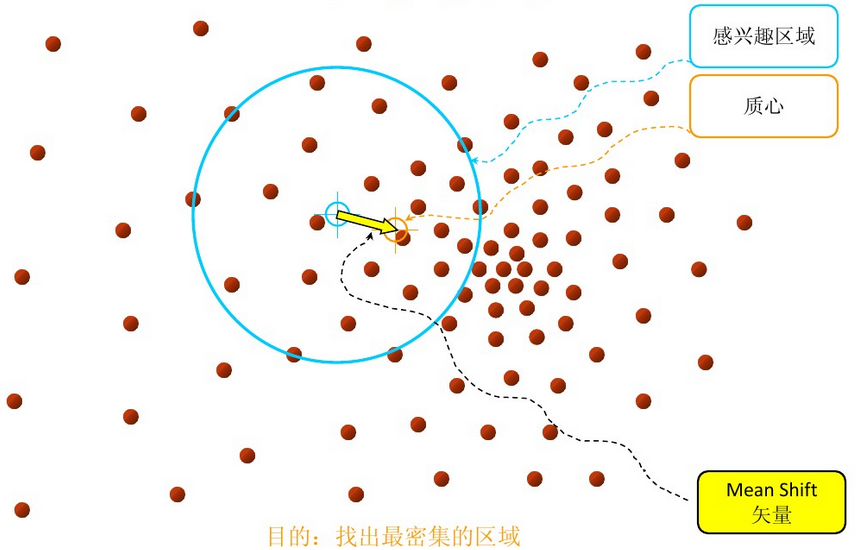
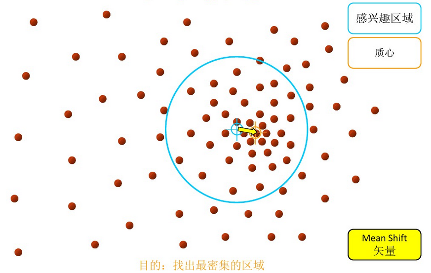
步骤2：移动该点到偏移均值点处（如图，其中黄色箭头就是M_h（meanshift向量））

再以meanshift向量的终点为圆心，再做一个高维的球。如下图所以，重复以上步骤，就可得到一个meanshift向量。如此重复下去，meanshift算法可以收敛到概率密度最大得地方。也就是最稠密的地方。

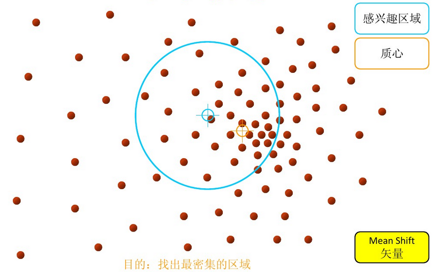
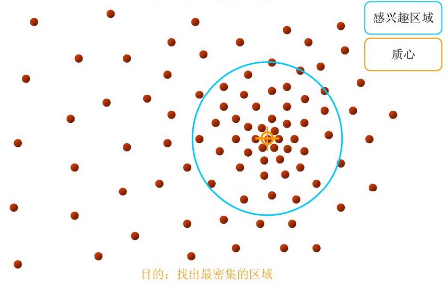
步骤3： 重复上述的过程(计算新的偏移均值，移动)

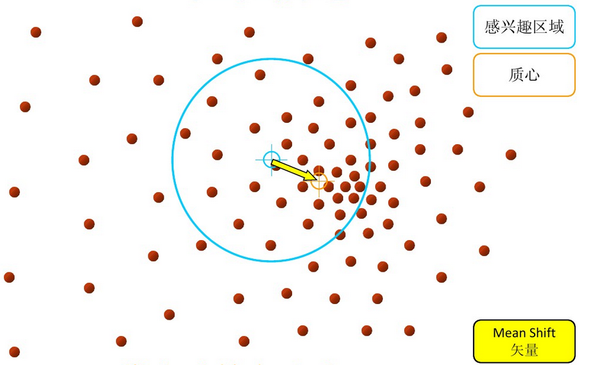
步骤4： 满足最终的条件，即退出。下图便是最终的结果！

从上述过程可以看出，在Mean Shift算法中，最关键的就是计算每个点的偏移均值，然后根据新计算的偏移均值更新点的位置。

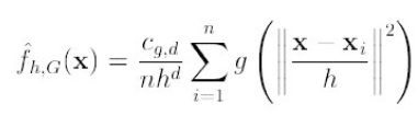
2.2.2、基本的Mean Shift向量形式

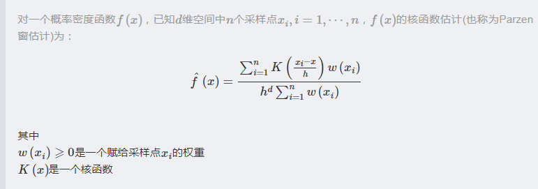
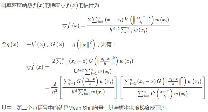
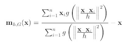
2.2.3、改进的Mean Shift向量形式

2.3、Mean Shift算法的解释

在Mean Shift算法中，实际上是利用了概率密度，求得概率密度的局部最优解。

2.3.1、概率密度梯度

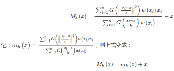
2.3.2、Mean Shift向量的修正

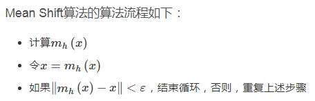
2.4、Mean Shift算法流程

--------------------------------------------------------------------------------------------------------------------------------分割线（始）----------------------------------------------------------------------------------------------------------------------------------

附：

关于Mean Shift的推导，再来一个版本。总结在这里便于对比。也可以去看原文：http://www.cnblogs.com/liqizhou/archive/2012/05/12/2497220.html

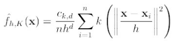
首先，通过核函数等，将meanshift算法变形为：

（1）

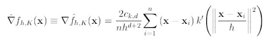
K()是核函数，h为半径，C_k,d/nh^d  为单位密度，要使得上式f得到最大，最容易想到的就是对上式进行求导，的确meanshift就是对上式进行求导：

（2）

令：

K(x)叫做g(x)的影子核，名字听上去挺深奥的，也就是求导的负方向，那么上式可以表示为：

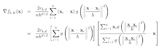
对于上式，如果才用高斯核，那么，第一项就等于f_h,k

第二项就相当于一个meanshift向量的式子：

那么（2）就可以表示为

下图分析的构成，如图，可以很清晰的表达其构成。

要使得=0，当且仅当=0，可以得出新的圆心坐标：

    （3）    

上面介绍了meanshift的流程，下面具体给出它的算法流程。

1. 选择空间中x为圆心，以h为半径为半径，做一个高维球，落在所有球内的所有点x_i
2. 计算，如果<ε(人工设定)，推出程序。如果>ε, 则利用（3）计算x，返回1。

下面介绍meashift算法怎样运用到图像上的聚类和跟踪：

一般一个图像就是个矩阵，像素点均匀的分布在图像上，就没有点的稠密性。所以怎样来定义点的概率密度，这才是最关键的。

如果我们就算点x的概率密度，采用的方法如下：以x为圆心，以h为半径。落在球内的点位x_i   定义二个模式规则。

（1）x像素点的颜色与x_i像素点颜色越相近，我们定义概率密度越高。

（2）离x的位置越近的像素点x_i，定义概率密度越高。

所以定义总的概率密度，是二个规则概率密度乘积的结果，可以用公式（4）表示：

（4）

其中：代表空间位置的信息，离远点越近，其值就越大，表示颜色信息，颜色越相似，其值越大。如图左上角图片，按照（4）计算的概率密度如图右上。利用meanshift对其聚类，可得到左下角的图。

 

--------------------------------------------------------------------------------------------------------------------------------分割线（末）----------------------------------------------------------------------------------------------------------------------------------

三、实验

3.1、实验数据

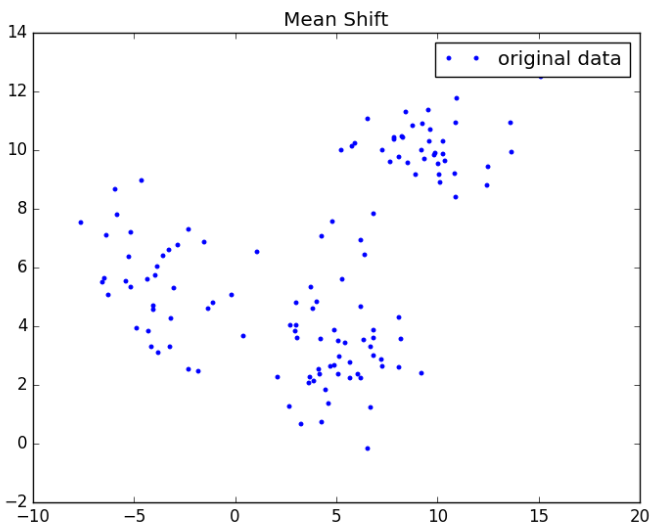
附上画图的python代码（注意，需要相应路径存放data）：

import matplotlib.pyplot as plt

f = open("data")
x = []
y = []
for line in f.readlines():
    lines = line.strip().split("	")
    if len(lines) == 2:
        x.append(float(lines[0]))
        y.append(float(lines[1]))
f.close()  

plt.plot(x, y, 'b.', label="original data")
plt.title('Mean Shift')
plt.legend(loc="upper right")
plt.show()

3.2 实验源码

import math
import sys
import numpy as np

MIN_DISTANCE = 0.000001#mini error

def load_data(path, feature_num=2):
    f = open(path)
    data = []
    for line in f.readlines():
        lines = line.strip().split("	")
        data_tmp = []
        if len(lines) != feature_num:
            continue
        for i in range(feature_num):
            data_tmp.append(float(lines[i]))

        data.append(data_tmp)
    f.close()
    return data

def gaussian_kernel(distance, bandwidth):
    m = np.shape(distance)[0]
    right = np.mat(np.zeros((m, 1)))
    for i in range(m):
        right[i, 0] = (-0.5 * distance[i] * distance[i].T) / (bandwidth * bandwidth)
        right[i, 0] = np.exp(right[i, 0])
    left = 1 / (bandwidth * math.sqrt(2 * math.pi))

    gaussian_val = left * right
    return gaussian_val

def shift_point(point, points, kernel_bandwidth):
    points = np.mat(points)
    m,n = np.shape(points)
    #计算距离
    point_distances = np.mat(np.zeros((m,1)))
    for i in range(m):
        point_distances[i, 0] = np.sqrt((point - points[i]) * (point - points[i]).T)

    #计算高斯核      
    point_weights = gaussian_kernel(point_distances, kernel_bandwidth)

    #计算分母
    all = 0.0
    for i in range(m):
        all += point_weights[i, 0]

    #均值偏移
    point_shifted = point_weights.T * points / all
    return point_shifted

def euclidean_dist(pointA, pointB):
    #计算pointA和pointB之间的欧式距离
    total = (pointA - pointB) * (pointA - pointB).T
    return math.sqrt(total)

def distance_to_group(point, group):
    min_distance = 10000.0
    for pt in group:
        dist = euclidean_dist(point, pt)
        if dist < min_distance:
            min_distance = dist
    return min_distance

def group_points(mean_shift_points):
    group_assignment = []
    m,n = np.shape(mean_shift_points)
    index = 0
    index_dict = {}
    for i in range(m):
        item = []
        for j in range(n):
            item.append(str(("%5.2f" % mean_shift_points[i, j])))

        item_1 = "_".join(item)
        print(item_1)
        if item_1 not in index_dict:
            index_dict[item_1] = index
            index += 1

    for i in range(m):
        item = []
        for j in range(n):
            item.append(str(("%5.2f" % mean_shift_points[i, j])))

            item_1 = "_".join(item)
        group_assignment.append(index_dict[item_1])

    return group_assignment

def train_mean_shift(points, kenel_bandwidth=2):
    #shift_points = np.array(points)
    mean_shift_points = np.mat(points)
    max_min_dist = 1
    iter = 0
    m, n = np.shape(mean_shift_points)
    need_shift = [True] * m

    #cal the mean shift vector
    while max_min_dist > MIN_DISTANCE:
        max_min_dist = 0
        iter += 1
        print ("iter : " + str(iter))
        for i in range(0, m):
            #判断每一个样本点是否需要计算偏置均值
            if not need_shift[i]:
                continue
            p_new = mean_shift_points[i]
            p_new_start = p_new
            p_new = shift_point(p_new, points, kenel_bandwidth)
            dist = euclidean_dist(p_new, p_new_start)

            if dist > max_min_dist:#record the max in all points
                max_min_dist = dist
            if dist < MIN_DISTANCE:#no need to move
                need_shift[i] = False

            mean_shift_points[i] = p_new
    #计算最终的group
    group = group_points(mean_shift_points)

    return np.mat(points), mean_shift_points, group

if __name__ == "__main__":
    #导入数据集
    path = "./data"
    data = load_data(path, 2)

    #训练，h=2
    points, shift_points, cluster = train_mean_shift(data, 2)

    for i in range(len(cluster)):
        print( "%5.2f,%5.2f	%5.2f,%5.2f	%i" % (points[i,0], points[i, 1], shift_points[i, 0], shift_points[i, 1], cluster[i]))

3.3 实验结果

经过Mean Shift算法聚类后的数据如下所示：

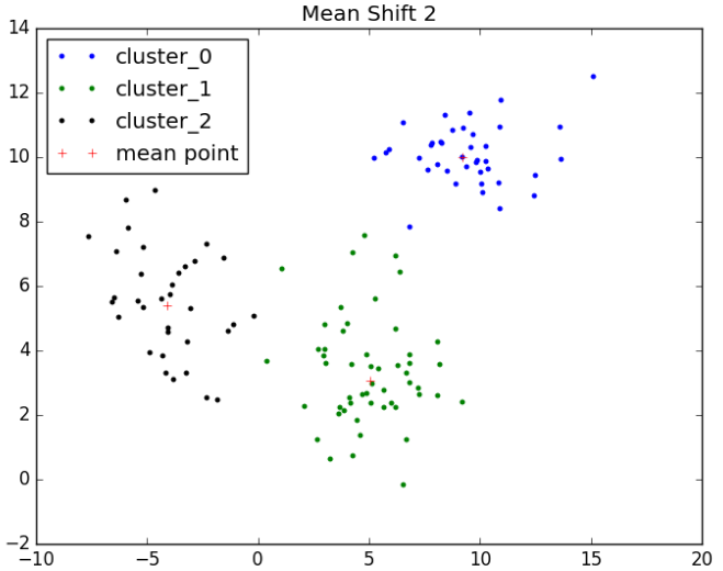
import matplotlib.pyplot as plt

f = open("data_mean")
cluster_x_0 = []
cluster_x_1 = []
cluster_x_2 = []
cluster_y_0 = []
cluster_y_1 = []
cluster_y_2 = []
center_x = []
center_y = []
center_dict = {}

for line in f.readlines():
    lines = line.strip().split("	")
    if len(lines) == 3:
        label = int(lines[2])
        if label == 0:
            data_1 = lines[0].strip().split(",")
            cluster_x_0.append(float(data_1[0]))
            cluster_y_0.append(float(data_1[1]))
            if label not in center_dict:
                center_dict[label] = 1
                data_2 = lines[1].strip().split(",")
                center_x.append(float(data_2[0]))
                center_y.append(float(data_2[1]))
        elif label == 1:
            data_1 = lines[0].strip().split(",")
            cluster_x_1.append(float(data_1[0]))
            cluster_y_1.append(float(data_1[1]))
            if label not in center_dict:
                center_dict[label] = 1
                data_2 = lines[1].strip().split(",")
                center_x.append(float(data_2[0]))
                center_y.append(float(data_2[1]))
        else:
            data_1 = lines[0].strip().split(",")
            cluster_x_2.append(float(data_1[0]))
            cluster_y_2.append(float(data_1[1]))
            if label not in center_dict:
                center_dict[label] = 1
                data_2 = lines[1].strip().split(",")
                center_x.append(float(data_2[0]))
                center_y.append(float(data_2[1]))    
f.close()


plt.plot(cluster_x_0, cluster_y_0, 'b.', label="cluster_0")
plt.plot(cluster_x_1, cluster_y_1, 'g.', label="cluster_1")
plt.plot(cluster_x_2, cluster_y_2, 'k.', label="cluster_2")
plt.plot(center_x, center_y, 'r+', label="mean point")
plt.title('Mean Shift 2')
#plt.legend(loc="best")
plt.show()

推荐链接：

https://blog.csdn.net/ttransposition/article/details/38514127

https://spin.atomicobject.com/2015/05/26/mean-shift-clustering/

https://github.com/mattnedrich/MeanShift_py