Pytorch学习-线性回归

简化模型：

• 假设1：影响房价的关键因素是卧室个数，卫生间个数和居住面积，记为x1,x2,x3
• 假设2：成交价是关键因素的加权和。
  y = w1x1+w2x2+w3x3
  权重和偏差的实际值在后面决定

线性模型

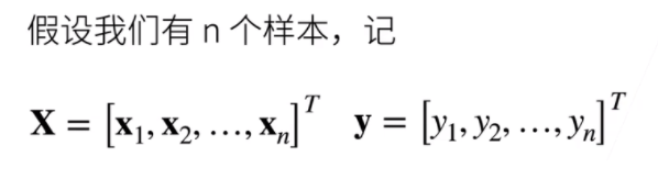
• 给定n维输入x = [x1,x2,...,xn]^T
• 线性模型有一个n维权重和一个标量偏差 w = [w1,w2,...,wn]^T,b
• 输出是输入的加权和 y = w1x1+w2x2+...+wnxn+b
• 向量版本 y = <w,x>+b

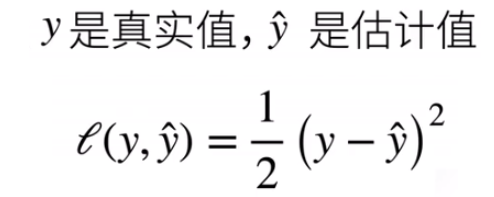
平方损失

训练数据

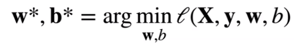
参数学习

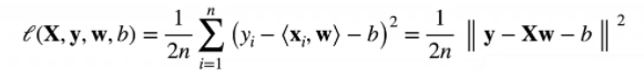
• 训练损失

• 最小化损失学习参数

总结

• 线性回归是对n维输入的加权，外加偏差
• 使用平方损失来衡量预测值和真实值的差异
• 线性回归有显示解
• 线性回归可以看做是单层神经网络

基础优化算法

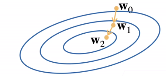
梯度下降

• 挑选一个初始值 w0
• 重复迭代参数t = 1,2,3

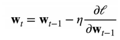
- 沿梯度方向将增加损失函数值
- 学习率：步长的超参数

小批量随机梯度下降

• 在整个训练集上算梯度太贵
  一个深度神经网络模型可能需要数分钟至数小时
• 我们可以随机采样b个样本i1,i2,...,ib来近似损失

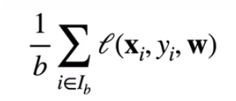
b是批量大小，另一个重要的超参数

线性回归从零开始实现

从零开始实现整个方法，包括数据流水线、模型、损失函数和小批量随机梯度下降优化器。

%matplotlib inline
import random #随机梯度权重
import torch
from d2l import torch as d2l

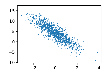
根据带有噪声的线性模型构造一个人造数据集。我们使用线性模型参数w = [2,-3.4]^T、b = 4.2和噪声项ε生成数据集及其标签：

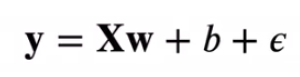
def synthetic_data(w,b,num_examples):
    '''生成y = Xw + b + 噪声。'''
    X = torch.normal(0,1,(num_examples,len(w)))#均值为零，方差为1的随机数
    y = torch.matmul(X,w)+ b
    y += torch.normal(0,0.01,y.shape)#均值为零，方差为0.01的随机噪音
    return X,y.reshape((-1,1))#-1表示由pytorch自动推导，1表示固定，即列向量为1

true_w = torch.tensor([2,-3.4])
true_b = 4.2
features,labels = synthetic_data(true_w,true_b,1000)

features中的每一行都包含一个二维数据样本，labels中每一行都包含一维标签值（一个标量）

print('features:',features,'
label:',labels[0])

features: tensor([[ 0.7857,  0.0540],
        [ 1.4230,  1.9870],
        [-0.2214,  1.6215],
        ...,
        [-1.2081, -0.4113],
        [ 1.7863,  3.8525],
        [ 0.8111,  0.7033]]) 
label: tensor([5.5789])

d2l.set_figsize()
# detach()表示分离出数值，不再含有梯度
d2l.plt.scatter(features[:,(1)].detach().numpy(),labels.detach().numpy(),1)

<matplotlib.collections.PathCollection at 0x20c603fcc70>

​

定义一个data_iter函数，该函数接收批量大小、特征矩阵和标签向量作为输入，生成大小为batch_size的小批量

def data_iter(batch_size,features,labels):
    num_examples = len(features)
    #设置索引
    indices = list(range(num_examples))
    #这些样本都是随机读取的，没有特定的顺序，需要打乱下标
    random.shuffle(indices)
    for i in range(0,num_examples,batch_size):
        batch_indices = torch.tensor(indices[i:min(i+
                                                   batch_size,num_examples)])
        yield features[batch_indices],labels[batch_indices]

batch_size = 10
for X,y in data_iter(batch_size,features,labels):
    print(X,'
',y)
    break

tensor([[-0.5396,  1.0611],
        [-0.3577, -0.4951],
        [-2.3002,  1.9732],
        [-0.7790, -0.1243],
        [ 1.4211, -2.1745],
        [-0.3561, -0.2842],
        [-0.8443, -0.0471],
        [ 0.0722, -0.3774],
        [-1.7615,  0.2300],
        [-0.9065, -3.0624]]) 
 tensor([[-0.4882],
        [ 5.1640],
        [-7.1245],
        [ 3.0805],
        [14.4374],
        [ 4.4567],
        [ 2.6782],
        [ 5.6375],
        [-0.1057],
        [12.8029]])

定义初始化模型参数

w = torch.normal(0,0.01,size=(2,1),requires_grad = True)
b = torch.zeros(1,requires_grad = True)

定义模型

def linreg(X,w,b):
    '''线性回归模型。'''
    return torch.matmul(X,w) + b

定义损失函数

def squared_loss(y_hat,y):
    '''均方损失。'''
    return (y_hat-y.reshape(y_hat.shape))**2/2

定义优化算法

def sgd(params,lr,batch_size):
    '''小批量随机梯度下降'''
    with torch.no_grad():
        for param in params:
            param -= lr * param.grad / batch_size
            param.grad.zero_()

训练过程

lr = 0.03 #学习率
num_epochs = 3 #扫描次数
net = linreg 
loss = squared_loss

for epoch in range(num_epochs):
    for X,y in data_iter(batch_size,features,labels):
        l = loss(net(X,w,b),y) # X和y的小批量损失
        # 因为l形状是（batch_size,1），而不是一个标量，l中的所有元素被加到
        #并以此计算关于[ w,b ]的梯度
        l.sum().backward()
        sgd([w,b],lr,batch_size) 
    with torch.no_grad():
        train_l = loss(net(features,w,b),labels)
        print(f'epoch{epoch+1},loss{float(train_l.mean()):f}')

epoch1,loss0.038016
epoch2,loss0.000143
epoch3,loss0.000050

比较真实参数和通过训练学到的参数来评估训练的成功程度

print(f'w的估计误差：{true_w - w.reshape(true_w.shape)}')
print(f'b的估计误差：{true_b - b}')

w的估计误差：tensor([ 0.0007, -0.0002], grad_fn=<SubBackward0>)
b的估计误差：tensor([0.0008], grad_fn=<RsubBackward1>)

线性回归的简洁实现

通过使用深度学习框架简介实现线性回归模型生成数据集

import numpy as np
import torch
from torch.utils import data
from d2l import torch as d2l

true_w = torch.tensor([2,-3.4])
true_b = 4.2
features,labels = d2l.synthetic_data(true_w,true_b,batch_size)

def load_array(data_arrays,batch_size,is_train = True):
    '''构造一个PyTorch数据迭代器'''
    dataset = data.TensorDataset(*data_arrays)#将两类数据一一对应
    return data.DataLoader(dataset,batch_size,shuffle = is_train)#重新排序
batch_size = 10
data_iter = load_array((features,labels),batch_size)

next(iter(data_iter))

[tensor([[ 1.3788, -1.2938],
         [-0.5648,  0.3607],
         [-1.4867, -0.7318],
         [-1.3304,  0.0436],
         [-1.0882, -0.6597],
         [ 2.4002,  1.1828],
         [ 0.7691, -0.8790],
         [-0.2221, -1.0182],
         [-0.5332, -0.6340],
         [-0.2190, -0.0083]]),
 tensor([[11.3507],
         [ 1.8421],
         [ 3.7258],
         [ 1.3721],
         [ 4.2723],
         [ 4.9844],
         [ 8.7432],
         [ 7.2262],
         [ 5.2892],
         [ 3.7768]])]

使用框架的预定好的层

# `nn`是神经网络的缩写
from torch import nn

net = nn.Sequential(nn.Linear(2,1))

初始化模型参数

net[0].weight.data.normal_(0,0.01)
net[0].bias.data.fill_(0)

tensor([0.])

均方误差

loss = nn.MSELoss()

实例化sgd

trainer = torch.optim.SGD(net.parameters(),lr = 0.03)#至少传入两个参数

训练过程

num_epochs = 3
for epoch in range(num_epochs):
    for X,y in data_iter:
        l = loss(net(X),y)
        trainer.zero_grad()
        l.backward()
        trainer.step()
    l = loss(net(features),labels)
    print(f'epoch {epoch+1}，loss {1:f}')

epoch 1，loss 1.000000
epoch 2，loss 1.000000
epoch 3，loss 1.000000