Sener O. and Koltun V. Multi-task learning as multi-objective optimization. In Advances in Neural Information Processing Systems (NIPS), 2018.
概
本文提出的 MGDA-UB 用于同时处理\(T\)个任务:
\[\tag{1}
\min_{\theta^{sh}, \: \theta^1, \cdots, \theta^T} \mathbf{L}(\theta^{sh}, \theta^1, \cdots, \theta^T) := (\hat{\mathcal{L}}^1(\theta^{sh}, \theta^1), \cdots, \hat{\mathcal{L}}^T(\theta^{sh}, \theta^T))^{\mathbf{T}}.
\]
其中
\[\hat{\mathcal{L}}^t(\theta^{sh}, \theta^t) := \frac{1}{N} \sum_i \mathcal{L}(f^t(x_i; \theta^{sh}, \theta^t), y_i^t), \: t =1,2,\cdots, T
\]
共享参数\(\theta^{sh}\)同时具备独立的参数\(\theta^t\).
在了解 MGDA-UB 之前, 务必先了解 MGDA.
主要内容
Pareto 最优
一种通常的同时解决多个任务的方法是施加不同的权重:
\[\min_{\theta} \sum_{t=1}^T c^t \hat{\mathcal{L}}^t.
\]
但对于\(\theta\)和\(\bar{\theta}\), 倘若满足
\[\hat{\mathcal{L}}^{t_1}(\theta) < \hat{\mathcal{L}}^{t_1}(\bar{\theta}) \\
\hat{\mathcal{L}}^{t_2}(\theta) > \hat{\mathcal{L}}^{t_2}(\bar{\theta}),
\]
该如何判断\(\theta, \bar{\theta}\)的优劣呢? 这个可能得根据一些其它的指标来判断了. MGDA所希望的是优化得到多个模型的 Pareto 最优解\(\theta^*\), 即不存在 \(\theta\) 满足
\[\hat{\mathcal{L}}^{t}(\theta^*) \ge \hat{\mathcal{L}}^t(\theta) \quad \forall t \\
\hat{\mathcal{L}}^{t}(\theta^*) > \hat{\mathcal{L}}^t(\theta) \quad \exist t.
\]
显然在 Pareto 最优的意义下, 我们找不到更好的解完全优于 \(\theta^*\).
KKT 条件
我们可以得到 (1) 的 KKT 条件:
\[\sum_{i=1}^T \alpha_i^t \nabla_{\theta^{sh}} \hat{\mathcal{L}}^t (\theta^{sh}, \theta^t) = 0, \\
\nabla_{\theta^t} \hat{\mathcal{L}}^t (\theta^{sh}, \theta^t) = 0, \: \forall t=1,2\cdots, T, \\
\sum_{i=1}^T \alpha_i = 1, \: \alpha_i \ge 0, \: \forall t = 1,2,\cdots, T.
\]
一个不严格的推导:
假设在 Pareto 最优解 \(\theta^*\) 下:
\[\hat{\mathcal{L}}^t(\theta^*) = C_t, \: t=1,2,\cdots, T.
\]
则
\[\begin{array}{rl}
\min_{\theta} & \hat{\mathcal{L}}^1 \\
\mathrm{s.t.} & \hat{\mathcal{L}}^t \le C_t, \: t=2,3,\cdots, T.
\end{array}
\]
则引入拉格朗日乘子 \(\lambda_t \ge 0\)可得
\[L(\theta; \lambda) =
\hat{\mathcal{L}}^1 +
\sum_{t=2}^T \lambda_t (\hat{\mathcal{L}}^t - C_t),
\]
通过
\[\nabla_{\theta} L = 0, \\
\alpha_t = \frac{\lambda_t}{\sum_t \lambda_t}, \: \lambda_1 = 1
\]
便可得到上方的关系.
MDGA-UB
因为\(\theta^{sh}\)和\(\theta^t\)之间是独立的, 所以对于后者我们可以利用普通的梯度即可, 对于前者, 本文利用 MGDA-UB 来选择合适的下降方向.
定义
\[V = \Bigg\{ \sum_{t=1}^T \alpha^t \nabla_{\theta^{sh}} \hat{\mathcal{L}}^t : \sum_t \alpha_t = 1, \alpha_t \ge 0 \: \forall t \Bigg\}.
\]
MGDA 中指出, 若
\[\tag{2}
v := \mathop{\text{argmin}}_{v \in V} \|v\|_2^2,
\]
则 \(-v\)是\(\theta^{sh}\)的一个可行的下降方向.
所以, 现在的问题是如何求解\(v\)呢?
特殊的双重任务
对于\(T=2\)的情形, (2) 等价于
\[\min_{\gamma \in [0, 1]} \:
\|
\gamma \nabla_{\theta^{sh}} \hat{\mathcal{L}}^1(\theta^{sh}, \theta^1)
+(1 - \gamma) \nabla_{\theta^{sh}} \hat{\mathcal{L}}^1(\theta^{sh}, \theta^1)
\|_2^2,
\]
其解可以显示表达为 (证明比较简单, 这里不写了)
\[\hat{\gamma} = \max(\min([\frac{(u_1 - u_2)^T u_2}{\|u_1 - u_2\|_2^2}], 1), 0).
\]
其中 \(u_t := \nabla_{\theta^{sh}} \hat{\mathcal{L}}^t(\theta^{sh}, \theta^t)\).

一般的多重任务
令
\[U = [u_1, u_2, \cdots, u_T], \: u_t := \nabla_{\theta^{sh}} \hat{\mathcal{L}}^t(\theta^{sh}, \theta^t).
\]
则 (2) 等价于
\[\begin{array}{rl}
\min_{\alpha} & \bm{\alpha}^T U^TU \bm{\alpha} \\
\mathrm{s.t.} & -\bm{\alpha} \preceq 0, \bm{1}^T \bm{\alpha} = 1.
\end{array}
\]
作者采用 Frank-Wolfe 算法来近似求解:
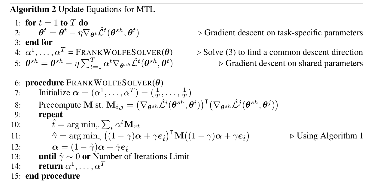
更高效
上述的算法在时间复杂度上有缺陷, 因为这要求我们对每一个任务 \(\hat{\mathcal{L}}^t\)分别回传梯度, 这会比较耗时. 但对于 Encoder-Decoder 类型的结构, 时间能够进一步减少:
\[f^t(x;\theta^{sh}, \theta^t) = (f^t(\cdot;\theta^t) \circ g(\cdot;\theta^{sh}))(x) = f(g(x; \theta^{sh}); \theta^t).
\]
令 \(Z = (z_1, z_2, \cdots, z_N)\)为encoder \(g\)所输出的隐变量, 则
\[\|\sum_{t=1}^T \alpha^t \nabla_{\theta^{sh}} \hat{\mathcal{L}}^t (\theta^{sh}, \theta^t)\|_2^2
\le \|\frac{\partial Z}{\partial \theta^{sh}}\|_2^2 \cdot \|\sum_{t=1}^T \alpha^t \nabla_{Z} \hat{\mathcal{L}}^t (\theta^{sh}, \theta^t)\|_2^2,
\]
故我们通过
\[\|\sum_{t=1}^T \alpha^t \nabla_{Z} \hat{\mathcal{L}}^t (\theta^{sh}, \theta^t)\|_2^2
\]
来找到\(\alpha\), 由于这是一个上界, 所找到的下降方向也不会太差. 此外, 由于隐变量\(Z\)的维度一般远远小于网络的共享参数, 且回传梯度只需到中间结点, 故计算成本会省很多.
注: 作者实验发现, 优化上界比直接优化本身反而效果更好, 这可能和SGD以及Frank-Wolfe本身是近似算法有关系 (\(Z\)的维度小, 解的可能更好).
Frank-Wolfe
- 求解线性规划问题
\[\begin{array}{rl}
\min_x & f(x) \\
\mathrm{s.t.} & Ax \le b \\
& Mx = m.
\end{array}
\]
- 每一步求解一阶近似
\[\begin{array}{rl}
\min_{x_t} & f(x_{t-1}) + \nabla^{\mathbf{T}} f(x_{t-1}) (x_t - x_{t-1}) \Leftrightarrow \nabla^T f(x_{t-1}) x_t \\
\mathrm{s.t.} & Ax_t \le b \\
& Mx_t = m,
\end{array}
\]
得到该问题的精确解 \(y_{t}\), 以及下降方向 \(\Delta_t := y_{t} - x_{t - 1}\).
3. 计算最速下降步长
\[\gamma_t = \min_{\gamma \in [0, 1]} f(x_{t-1} + \gamma_t \cdot \Delta_t),
\]
- 更新 \(x_t = x_{t-1} + \gamma_t \Delta_t = \gamma_t y_t + (1 - \gamma_t)x_{t-1}\).
上文中的算法2可以据此一一对照得到.
实现细节
从代码中发现了一些细节:
- \(\gamma\) 取值 \([0.001, 0.999]\);
- 梯度用于算法二计算\(\alpha\)有可能会通过标准化;
- 得到\(\alpha\)之后作者scale每个损失, 再回传梯度, 也就是说即便上面用了标准化, 真正的梯度用的时候还是没标准化的.
代码
原文代码