目录:
(1)为什么使用attention
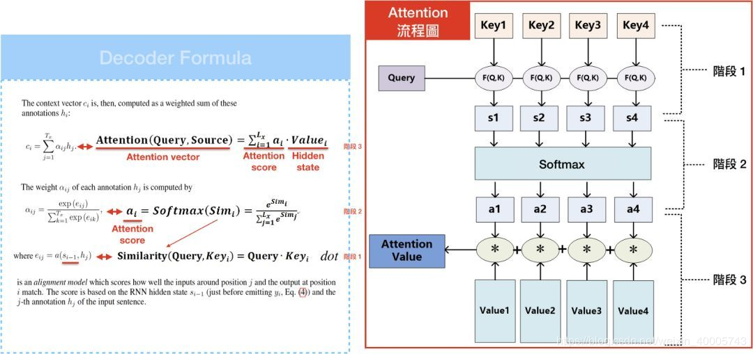
(2)attention的定义以及四种相似度计算方式
(3)attention类型(scaled dot-product attention multi-head attention)
(1)self-attention的计算
(2) self-attention如何并行
(3) self-attention的计算总结
(4) self-attention的类型(multi-head self-attention)
(1)传统的seq2seq
(2)seq2seq with attention
(1)整体结构
(2)细节:三种应用(encoder/decoder/encoder-decoder) + 位置encoding + 残差(Add) + Layer norm + 前馈神经网络(feed forward) + mask(decoder)
(3)实战
一. 前提:
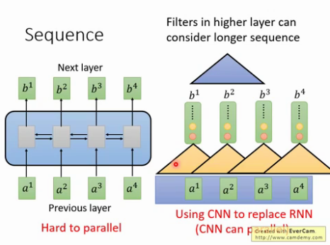
1. RNN : 解决INPUT是序列化的问题,但是RNN存在的缺陷是难以并行化处理.
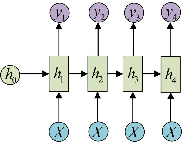
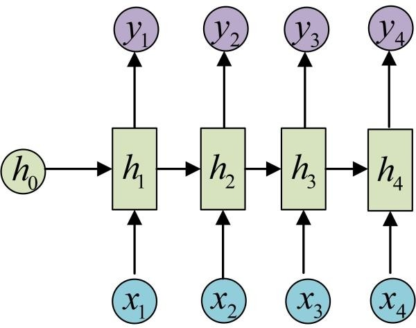
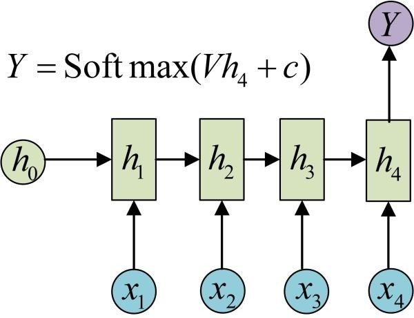
| (1) RNN(N vs N) | (2) RNN (N vs 1) | ||
|
|
|
||
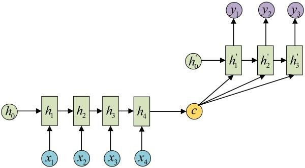
| (3) RNN (1 vs N) | (4) RNN (N vs M)---seq2seq | ||
 |
 |
||
2. CNN : 使用CNN来replaceRNN,可以并行,如下图每个黄色三角形都可以并行. 但是问题是难解决长依赖的序列, 解决办法是叠加多层的CNN,比如下图的CNN黄色三角形和蓝色三角形为两层CNN,
3. attention:
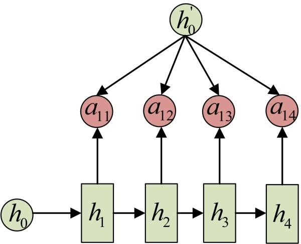
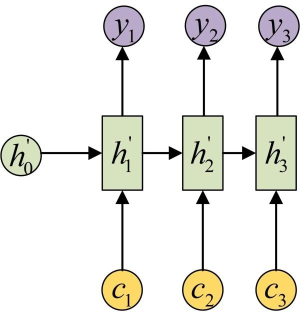
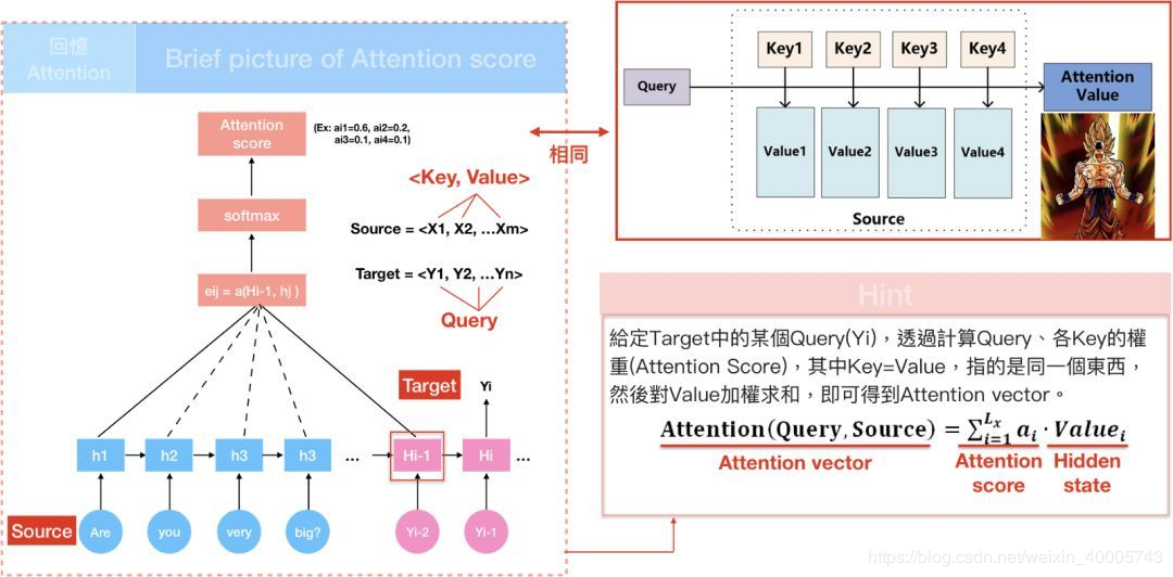
在Encoder-Decoder结构中,Encoder把所有的输入序列都编码成一个统一的语义特征c再解码,因此, c中必须包含原始序列中的所有信息,它的长度就成了限制模型性能的瓶颈。如机器翻译问题,当要翻译的句子较长时,一个c可能存不下那么多信息,就会造成翻译精度的下降。
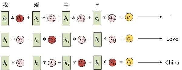
Attention机制通过在每个时间输入不同的c来解决这个问题,下图是Attention机制的encoder and Decoder:
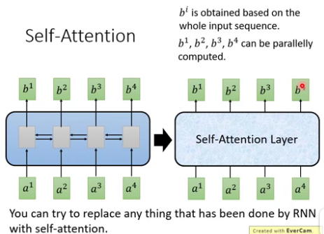
4. self-attention : 其输入和输出和RNN一样,就是中间不一样. 如下图, b1到b4是同时计算出来, RNN的b4必须要等到b1计算完.
二.Attention
1. 为什么要用attention model?
The attention model用来帮助解决机器翻译在句子过长时效果不佳的问题。并且可以解决RNN难并行的问题.
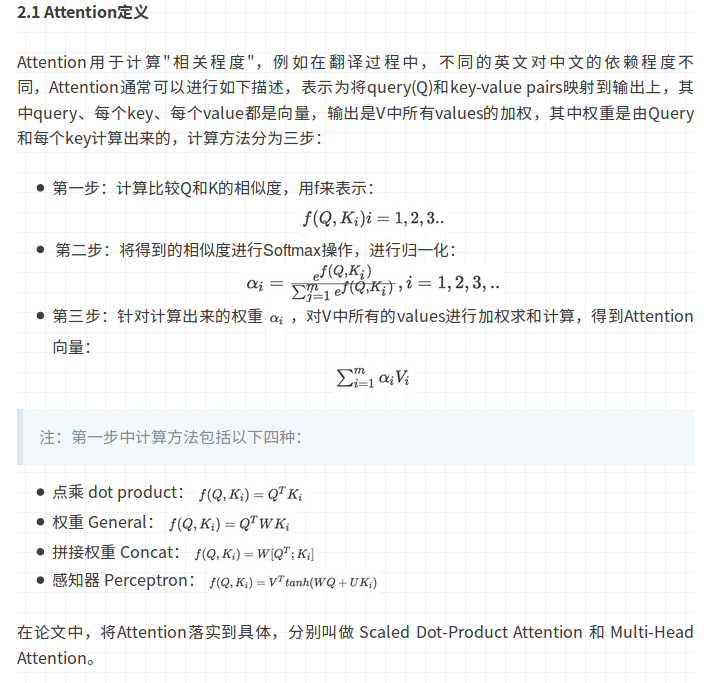
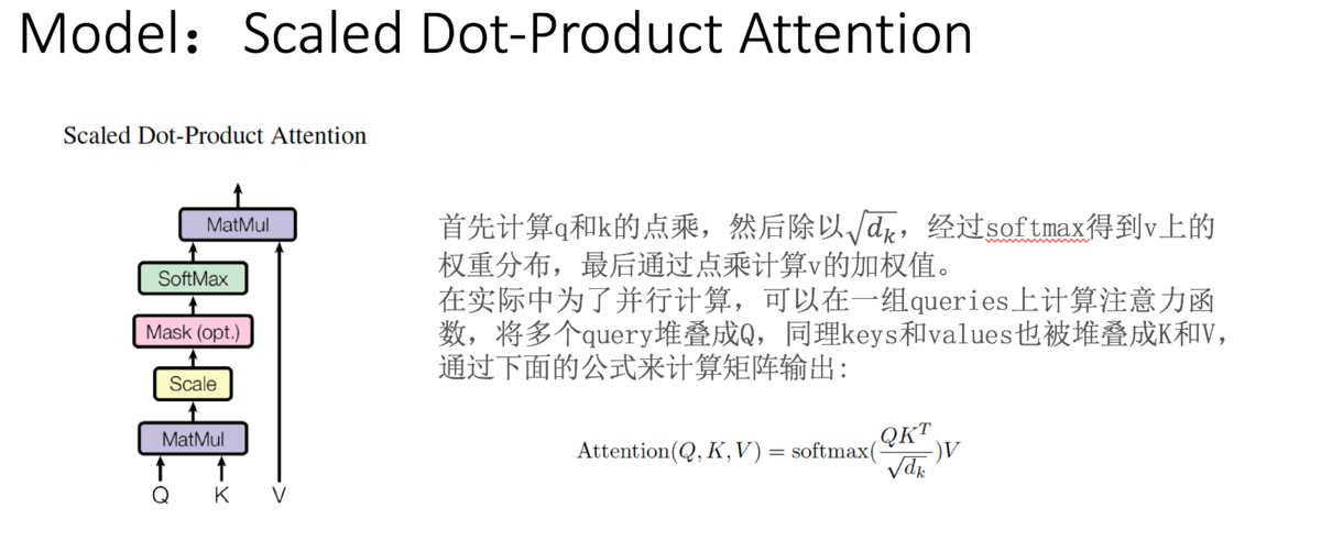
3. attentionl类型
点积注意力机制的优点是速度快、占用空间小。
三. self-attention
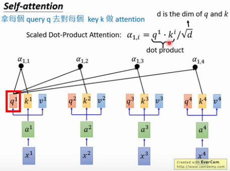
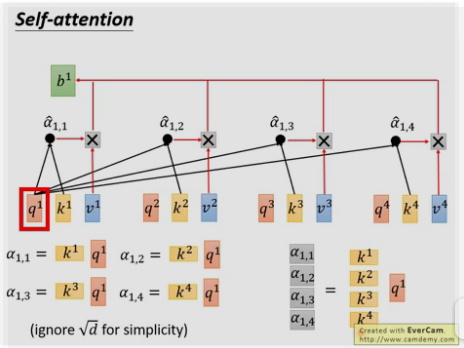
1. self-attention 的计算(Attention is all you need)

用每个query q去对每个key k做attention , 即计算得到α1,1 , α1,2 ……,
为什么要除以d [d等于q或k的维度,两者维度一样] ? 因为q和k的维度越大,dot product 之后值会更大,为了平衡值,相当于归一化这个值,除以一个d.

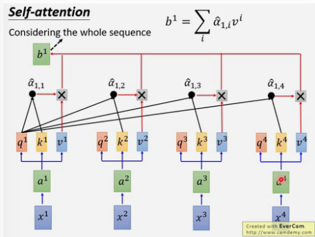
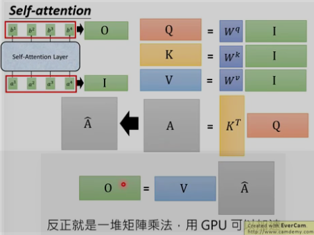
2. self-attention如何并行
self-attention最终为一些矩阵相乘的形式,可以采用并行方式来计算.

以上每个α都可以并行计算

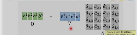
3. 计算总结:
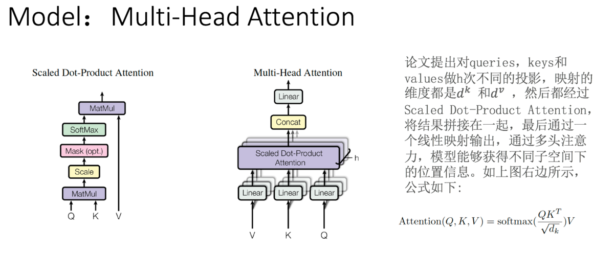
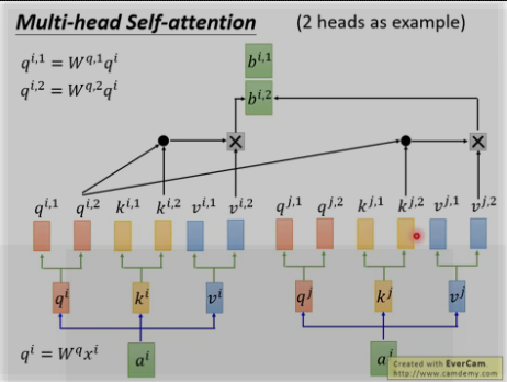
4. self_attention的类型
多头: 为何?因为不同的head可以关注不同的信息, 比如第一个head关注长时间的信息,第二个head关注短时间的信息.
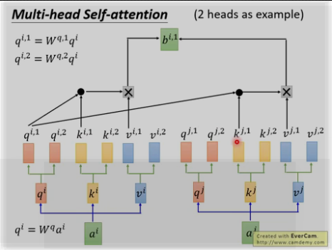
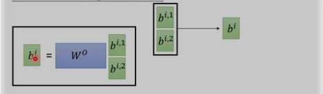
将两个bi,1和bi,2进行concat并乘以W0来降为成bi
四. seq2seq
传统的seq2seq: 中间用的是RNN
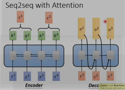
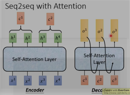
seq2seq with attention
五. Transformer
细扣 : https://mp.weixin.qq.com/s/RLxWevVWHXgX-UcoxDS70w
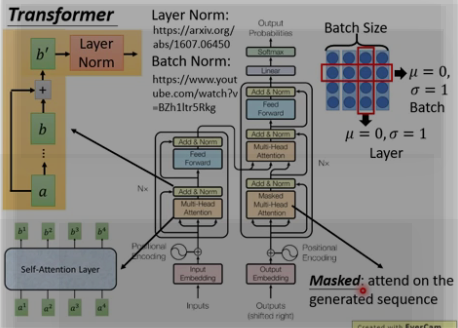
1. 整体架构:
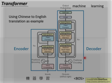
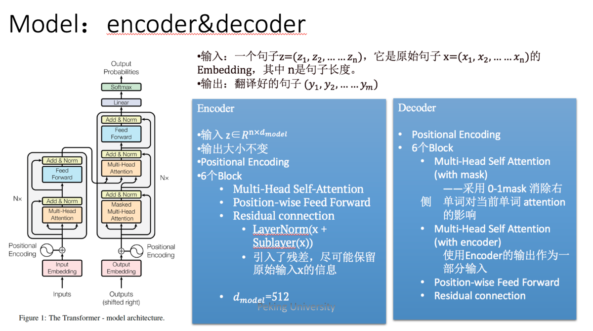
Transformer遵循这种结构,encoder和decoder都使用堆叠的self-attention和point-wise,fully connected layers。
Encoder: encoder由6个相同的层堆叠而成,每个层有两个子层。
第一个子层是多头自我注意力机制(multi-head self-attention mechanism),
第二层是简单的位置的全连接前馈网络(position-wise fully connected feed-forward network)。
中间: 两个子层中会使用一个残差连接,接着进行层标准化(layer normalization)。
也就是说每一个子层的输出都是LayerNorm(x + sublayer(x))。
网络输入是三个相同的向量q, k和v,是word embedding和position embedding相加得到的结果。为了方便进行残差连接,我们需要子层的输出和输入都是相同的维度。
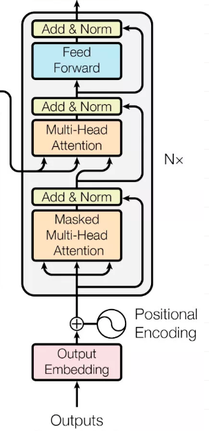
Decoder:
三层: (多头self-attention + 多头attention + feed-forword )
decoder也是由N(N=6)个完全相同的Layer组成,decoder中的Layer由encoder的Layer中插入一个Multi-Head Attention + Add&Norm组成。
输入 : 输出的embedding与输出的position embedding求和做为decoder的输入,
MA-1层: 经过一个Multi-HeadAttention + Add&Norm((MA-1)层,MA-1层的输出做为下一Multi-Head Attention + Add&Norm(MA-2)的query(Q)输入,
MA-2层的Key和Value输入(从图中看,应该是encoder中第i(i = 1,2,3,4,5,6)层的输出对于decoder中第i(i = 1,2,3,4,5,6)层的输入)。
MA-2层的输出输入到一个前馈层(FF), 层与层之间使用的Position-wise feed forward network,经过AN(Add&norm)操作后,经过一个线性+softmax变换得到最后目标输出的概率。
mask : 对于decoder中的第一个多头注意力子层,需要添加masking,确保预测位置i的时候仅仅依赖于位置小于i的输出。
2. trip细节
(1) 三种应用
Transformer会在三个不同的方面使用multi-head attention:
1. encoder-decoder attention:使用multi-head
attention,输入为encoder的输出和decoder的self-attention输出,其中encoder的self-attention作为
key and value,decoder的self-attention作为query
2. encoder self-attention:使用 multi-head attention,输入的Q、K、V都是一样的(input embedding and positional embedding)
3. decoder self-attention:在decoder的self-attention层中,deocder 都能够访问当前位置前面的位置
(2)位置encoding
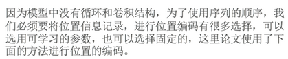
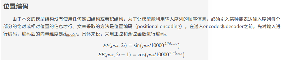
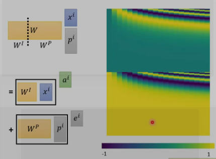
这样做的目的是因为正弦和余弦函数具有周期性,对于固定长度偏差k(类似于周期),post +k位置的PE可以表示成关于pos位置PE的一个线性变化(存在线性关系),这样可以方便模型学习词与词之间的一个相对位置关系。
上面的self-attention有个问题,q缺乏位置信息,因为近邻和长远的输入是同等的计算α.
位置encoding的ei是人工设置的,不是学习的.将其加入ai中.
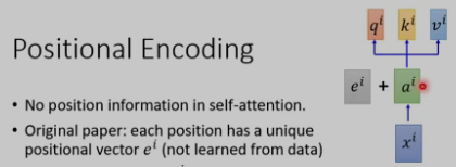
为何是和ai相加,而不是concat?
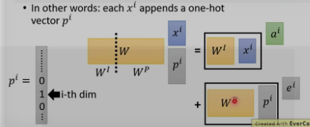
这里的Wp是通过别的方法计算的,如下图所示
(3) 残差
对于每个encoder里面的每个sub-layer,它们都有一个残差的连接,理论上这可以回传梯度.
这种方式理论上可以很好的回传梯度
作者:收到一只叮咚
链接:https://www.imooc.com/article/67493
来源:慕课网
(4) Layer Norm
每个sub-layer后面还有一步 layer-normalization [layer Norm一般和RNN相接] 。可以加快模型收敛速度.
Batch Norm和Layer Norm 的区别, 下图右上角, 横向为batch size取均值为0, sigma = 1. 纵向 为layer Norm , 不需要batch size.
(5) Position-wise feed forward network 前馈神经网络
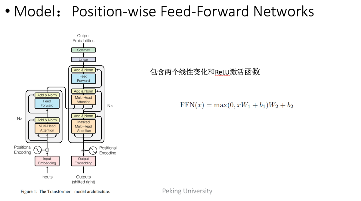
用了两层Dense层,activation用的都是Relu。
可以看成是两层的1*1的1d-convolution。hidden_size变化为:512->2048->512
Position-wise feed forward network,其实就是一个MLP 网络,1 的输出中,每个 d_model 维向量 x
在此先由 xW_1+b_1 变为 d_f $维的 x',再经过max(0,x')W_2+b_2 回归 d_model
维。之后再是一个residual connection。输出 size 仍是 $[sequence_length, d_model]$
(6) Masked : [decoder]
注意encoder里面是叫self-attention,decoder里面是叫masked self-attention。
这里的masked就是要在做language modelling(或者像翻译)的时候,不给模型看到未来的信息。

mask就是沿着对角线把灰色的区域用0覆盖掉,不给模型看到未来的信息。
(7) 优化
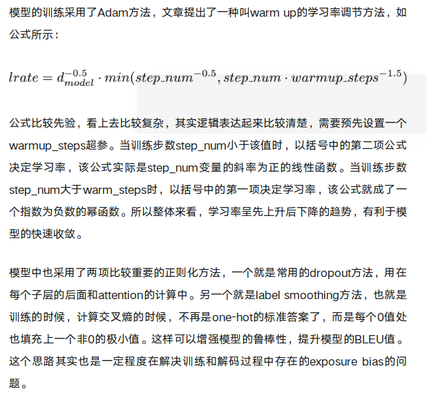
模型的训练采用了Adam方法,文章提出了一种叫warm up的学习率调节方法,如公式所示:
作者:收到一只叮咚
链接:https://www.imooc.com/article/67493
来源:慕课网
发展: universal transformer
应用: NLP self attention GAN (用在图像上)
3. 实战
https://www.jianshu.com/p/2b0a5541a17c
3.1 encoder
(1) 输入: encoder embedding和position embedding相加
(2) 两种attention
(3) Add & Normalize & FFN
3.2 decoder
(1)输入: decoder embedding和position embedding相加
(2)mask multi-head attention和encoder-decoder attention
(3)Add & Normalize & FFN & 输出
3.1 encoder
(1)输入: input embedding和position embedding相加
原始数据: word2vec [embedding表] + input_sentence [x] + output_sentence [y] + position embedding(固定)
①输入input_sentence [x] 和 word2vec [embedding表]
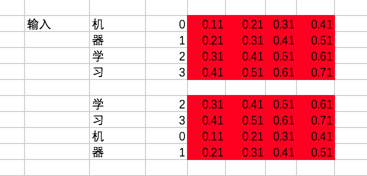
假设我们有两条训练数据(input_sentence [x]):
[机、器、学、习] -> [ machine、learning]
[学、习、机、器] -> [learning、machine]
encoder的输入在转换成id后变为[[0,1,2,3],[2,3,0,1]]。
接下来,通过查找中文的embedding表(word2vec),转换为embedding为:
②将position embedding设为固定值,但实际是通过三角函数来计算得到的,这里为了方便设为固定值,注意这个position embedding是不用迭代训练的:
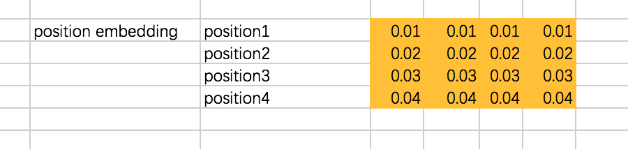
③对输入input_embedding加入位置偏置position_embedding,注意这里是两个向量的对位相加:
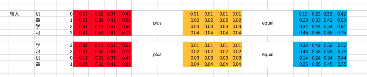
④output_sentence [y]和input_sentence做相同的处理
代码:


import tensorflow as tf

chinese_embedding = tf.constant([[0.11,0.21,0.31,0.41],
                         [0.21,0.31,0.41,0.51],
                         [0.31,0.41,0.51,0.61],
                         [0.41,0.51,0.61,0.71]],dtype=tf.float32)


english_embedding = tf.constant([[0.51,0.61,0.71,0.81],
                         [0.52,0.62,0.72,0.82],
                         [0.53,0.63,0.73,0.83],
                         [0.54,0.64,0.74,0.84]],dtype=tf.float32)


position_encoding = tf.constant([[0.01,0.01,0.01,0.01],
                         [0.02,0.02,0.02,0.02],
                         [0.03,0.03,0.03,0.03],
                         [0.04,0.04,0.04,0.04]],dtype=tf.float32)

encoder_input = tf.constant([[0,1,2,3],[2,3,0,1]],dtype=tf.int32)


with tf.variable_scope("encoder_input"):
    encoder_embedding_input = tf.nn.embedding_lookup(chinese_embedding,encoder_input)
    encoder_embedding_input = encoder_embedding_input + position_encoding


with tf.Session() as sess:
    sess.run(tf.global_variables_initializer())
    print(sess.run([encoder_embedding_input]))
(2) attention
[scaled dot-product attention]
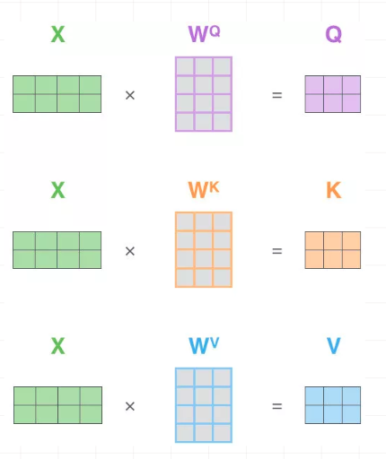
①计算Q . K . V [embedding × 三个W]
咱们先说说Q、K、V。比如我们想要计算上图中machine和机、器、学、习四个字的attention,并加权得到一个输出,那么Query由machine对应的embedding计算得到,K和V分别由机、器、学、习四个字对应的embedding得到。
在encoder的self-attention中,由于是计算自身和自身的相似度,所以Q、K、V都是由输入的embedding得到的,不过我们还是加以区分。
这里, Q、K、V分别通过一层全连接神经网络得到,同样,我们把对应的参数矩阵都写作常量。
接下来,以第一条输入为例, 将embedding 和 三个 W 矩阵相乘:
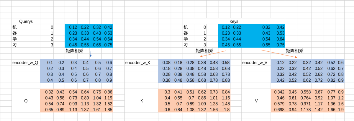
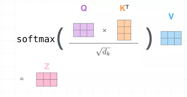
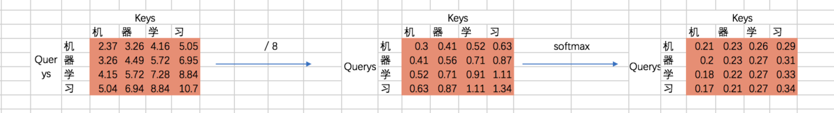
②计算α权重 [ softmax(Q * KT / sqrt(dk))]
计算Q和K的相关性大小,这里使用内积的方式,相当于QKT: (下图中V应该改成K,不影响整个过程理解),得到结果为attention map
机和机自身的相关性是2.37(未进行归一化处理),机和器的相关性是3.26,依次类推。
接着除以一个规范化因子,然后进行softmax操作,这里的规范化因子选择除以8,然后每行进行一个softmax归一化操作(按行做归一化是因为attention的初衷是计算每个Query和所有的Keys之间的相关性):
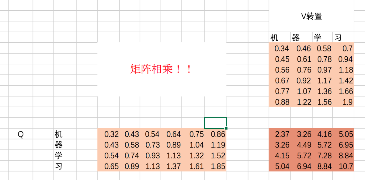
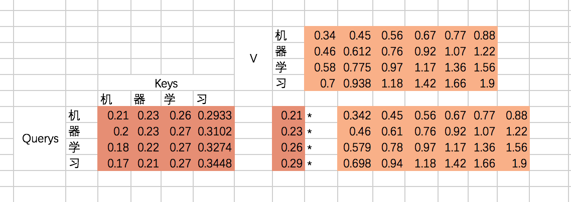
③将α 与V加权求和:
最后就是得到每个输入embedding 对应的输出embedding,也就是基于attention map对V进行加权求和,以“机”这个输入为例,最后的输出应该是V对应的四个向量的加权求和:
代码:
with tf.variable_scope("encoder_scaled_dot_product_attention"):
    encoder_Q = tf.matmul(tf.reshape(encoder_embedding_input,(-1,tf.shape(encoder_embedding_input)[2])),w_Q)
    encoder_K = tf.matmul(tf.reshape(encoder_embedding_input,(-1,tf.shape(encoder_embedding_input)[2])),w_K)
    encoder_V = tf.matmul(tf.reshape(encoder_embedding_input,(-1,tf.shape(encoder_embedding_input)[2])),w_V)

####① 计算Q K V
    encoder_Q = tf.reshape(encoder_Q,(tf.shape(encoder_embedding_input)[0],tf.shape(encoder_embedding_input)[1],-1))
    encoder_K = tf.reshape(encoder_K,(tf.shape(encoder_embedding_input)[0],tf.shape(encoder_embedding_input)[1],-1))
    encoder_V = tf.reshape(encoder_V,(tf.shape(encoder_embedding_input)[0],tf.shape(encoder_embedding_input)[1],-1))

 ####②计算α , softmax( Q * KT / sqrt(dk) )
    attention_map = tf.matmul(encoder_Q,tf.transpose(encoder_K,[0,2,1]))
    attention_map = attention_map / 8
    attention_map = tf.nn.softmax(attention_map)

###③ α * V ,自己补的,不一定对
    #### weightedSumV = tf.matmul(attention_map,encoder_V)


with tf.Session() as sess:
    sess.run(tf.global_variables_initializer())
    print(sess.run(attention_map))
    # print(sess.run(weightedSumV))
[multi-head attention]
Multi-Head Attention就是把Scaled Dot-Product Attention的过程做H次,然后把输出Z合起来。 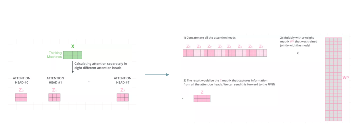
① 切分多个Head ( 即多个Q K V) , 并多次进行scaled dot-product attention
假设我们刚才计算得到的Q、K、V从中间切分,分别作为两个Head的输入:
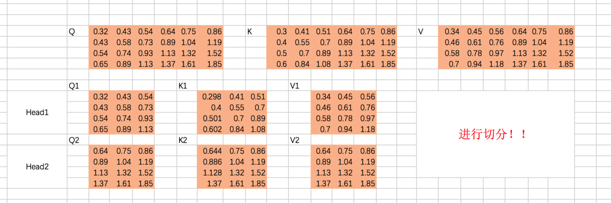
重复上面的Scaled Dot-Product Attention过程,我们分别得到两个Head的输出:

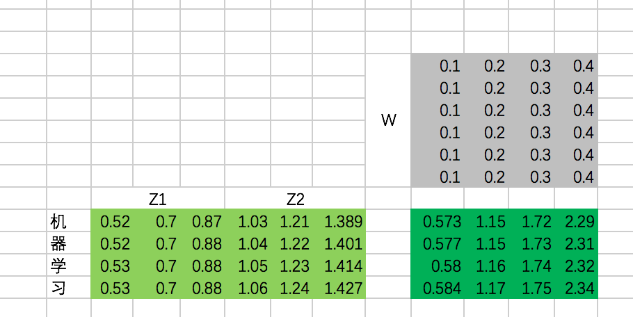
②concat多个Scaled Dot-Product Attention的结果 z , 并将其乘以W降维
接下来,我们需要通过一个权重矩阵,来得到最终输出。
为了我们能够进行后面的Add的操作,我们需要把输出的长度和输入保持一致,即每个单词得到的输出embedding长度保持为4。
同样,我们这里把转换矩阵W设置为常数:
代码:
w_Z = tf.constant([[0.1,0.2,0.3,0.4],
                   [0.1,0.2,0.3,0.4],
                   [0.1,0.2,0.3,0.4],
                   [0.1,0.2,0.3,0.4],
                   [0.1,0.2,0.3,0.4],
                   [0.1,0.2,0.3,0.4]],dtype=tf.float32)


with tf.variable_scope("encoder_input"):
    encoder_embedding_input = tf.nn.embedding_lookup(chinese_embedding,encoder_input)
    encoder_embedding_input = encoder_embedding_input + position_encoding

with tf.variable_scope("encoder_multi_head_product_attention"):
    encoder_Q = tf.matmul(tf.reshape(encoder_embedding_input,(-1,tf.shape(encoder_embedding_input)[2])),w_Q)
    encoder_K = tf.matmul(tf.reshape(encoder_embedding_input,(-1,tf.shape(encoder_embedding_input)[2])),w_K)
    encoder_V = tf.matmul(tf.reshape(encoder_embedding_input,(-1,tf.shape(encoder_embedding_input)[2])),w_V)

###① 生成Q K V
    encoder_Q = tf.reshape(encoder_Q,(tf.shape(encoder_embedding_input)[0],tf.shape(encoder_embedding_input)[1],-1))
    encoder_K = tf.reshape(encoder_K,(tf.shape(encoder_embedding_input)[0],tf.shape(encoder_embedding_input)[1],-1))
    encoder_V = tf.reshape(encoder_V,(tf.shape(encoder_embedding_input)[0],tf.shape(encoder_embedding_input)[1],-1))

###②最后一维切分 成多个Head ---Q K V
    encoder_Q_split = tf.split(encoder_Q,2,axis=2)
    encoder_K_split = tf.split(encoder_K,2,axis=2)
    encoder_V_split = tf.split(encoder_V,2,axis=2)

    ###第一维合并Q K V ,方便计算
    encoder_Q_concat = tf.concat(encoder_Q_split,axis=0)
    encoder_K_concat = tf.concat(encoder_K_split,axis=0)
    encoder_V_concat = tf.concat(encoder_V_split,axis=0)

    ###计算attention α
    attention_map = tf.matmul(encoder_Q_concat,tf.transpose(encoder_K_concat,[0,2,1]))
    attention_map = attention_map / 8
    attention_map = tf.nn.softmax(attention_map)

    ### α和V加权求和,结果为Z
    weightedSumV = tf.matmul(attention_map,encoder_V_concat)

###③ 将多个head求出来的Z合并
    outputs_z = tf.concat(tf.split(weightedSumV,2,axis=0),axis=2)

###④ 合并的Z与W相乘降维得到最终的Z
    outputs = tf.matmul(tf.reshape(outputs_z,(-1,tf.shape(outputs_z)[2])),w_Z)
    outputs = tf.reshape(outputs,(tf.shape(encoder_embedding_input)[0],tf.shape(encoder_embedding_input)[1],-1))

import numpy as np
with tf.Session() as sess:
#     print(sess.run(encoder_Q))
#     print(sess.run(encoder_Q_split))
    #print(sess.run(weightedSumV))
    #print(sess.run(outputs_z))
    print(sess.run(outputs))
更详细的解释split函数和concat函数
split函数主要有三个参数,第一个是要split的tensor,第二个是分割成几个tensor,第三个是在哪一维进行切分。也就是说, encoder_Q_split = tf.split(encoder_Q,2,axis=2),执行这段代码的话,encoder_Q这个tensor会按照axis=2切分成两个同样大的tensor,这两个tensor的axis=0和axis=1维度的长度是不变的,但axis=2的长度变为了一半,我们在后面通过图示的方式来解释。
从代码可以看到,共有两次split和concat的过程,第一次是将Q、K、V切分为不同的Head:
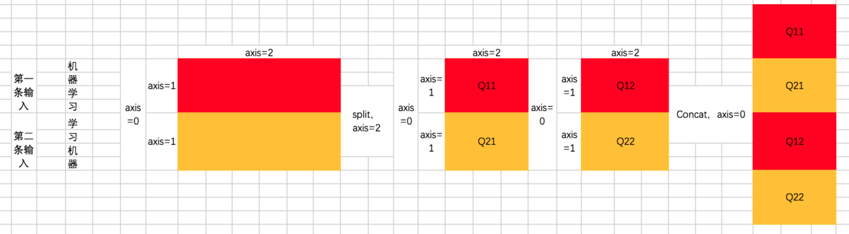
也就是说,原先每条数据的所对应的各Head的Q并非相连的,而是交替出现的,即 [Head1-Q11,Head1-Q21,Head2-Q12,Head2-Q22]
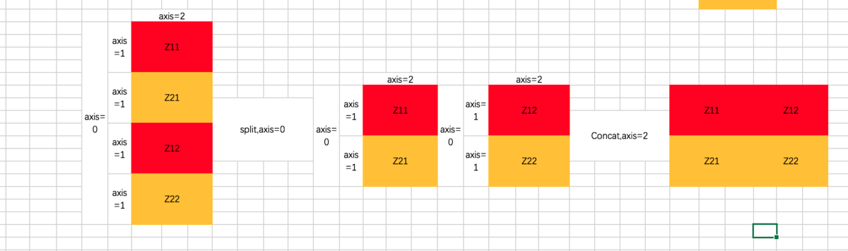
第二次是最后计算完每个Head的输出Z之后,通过split和concat进行还原,过程如下:
(3) Add & Normalize & FFN
第一次Add & Normalize:
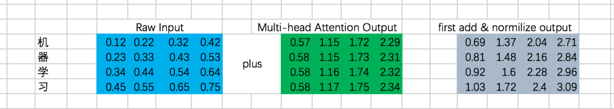
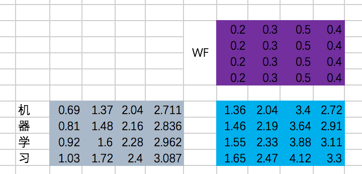
接下来是一个FFN,我们仍然假设是固定的参数,那么output是:
第二次Add & Normalize
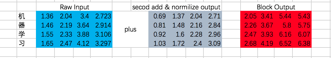
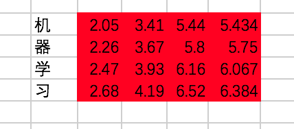
我们终于在经过一个Encoder的Block后得到了每个输入对应的输出,分别为:
代码:
with tf.variable_scope("encoder_block"):
    encoder_Q = tf.matmul(tf.reshape(encoder_embedding_input,(-1,tf.shape(encoder_embedding_input)[2])),w_Q)
    encoder_K = tf.matmul(tf.reshape(encoder_embedding_input,(-1,tf.shape(encoder_embedding_input)[2])),w_K)
    encoder_V = tf.matmul(tf.reshape(encoder_embedding_input,(-1,tf.shape(encoder_embedding_input)[2])),w_V)

    encoder_Q = tf.reshape(encoder_Q,(tf.shape(encoder_embedding_input)[0],tf.shape(encoder_embedding_input)[1],-1))
    encoder_K = tf.reshape(encoder_K,(tf.shape(encoder_embedding_input)[0],tf.shape(encoder_embedding_input)[1],-1))
    encoder_V = tf.reshape(encoder_V,(tf.shape(encoder_embedding_input)[0],tf.shape(encoder_embedding_input)[1],-1))

    encoder_Q_split = tf.split(encoder_Q,2,axis=2)
    encoder_K_split = tf.split(encoder_K,2,axis=2)
    encoder_V_split = tf.split(encoder_V,2,axis=2)

    encoder_Q_concat = tf.concat(encoder_Q_split,axis=0)
    encoder_K_concat = tf.concat(encoder_K_split,axis=0)
    encoder_V_concat = tf.concat(encoder_V_split,axis=0)

    attention_map = tf.matmul(encoder_Q_concat,tf.transpose(encoder_K_concat,[0,2,1]))
    attention_map = attention_map / 8
    attention_map = tf.nn.softmax(attention_map)

    #multi-head attention的计算结果
    weightedSumV = tf.matmul(attention_map,encoder_V_concat)

    outputs_z = tf.concat(tf.split(weightedSumV,2,axis=0),axis=2)

    #将多头结果的维度转为和encoder_embedding_input维度一样
    sa_outputs = tf.matmul(tf.reshape(outputs_z,(-1,tf.shape(outputs_z)[2])),w_Z)
    sa_outputs = tf.reshape(sa_outputs,(tf.shape(encoder_embedding_input)[0],tf.shape(encoder_embedding_input)[1],-1))

    ##第一次add
    sa_outputs = sa_outputs + encoder_embedding_input

    # todo :add BN
    W_f = tf.constant([[0.2,0.3,0.5,0.4],
                       [0.2,0.3,0.5,0.4],
                       [0.2,0.3,0.5,0.4],
                       [0.2,0.3,0.5,0.4]])
    ##FFN
    ffn_outputs = tf.matmul(tf.reshape(sa_outputs,(-1,tf.shape(sa_outputs)[2])),W_f)
    ffn_outputs = tf.reshape(ffn_outputs,(tf.shape(sa_outputs)[0],tf.shape(sa_outputs)[1],-1))

    #第二次add
    encoder_outputs = ffn_outputs + sa_outputs
    # todo :add BN

import numpy as np
with tf.Session() as sess:
#     print(sess.run(encoder_Q))
#     print(sess.run(encoder_Q_split))
    #print(sess.run(weightedSumV))
    #print(sess.run(outputs_z))
    #print(sess.run(sa_outputs))
    #print(sess.run(ffn_outputs))
    print(sess.run(encoder_outputs))
3.2 decoder
相比Encoder,这里的过程分为6步,分别是 masked multi-head self attention、Add & Normalize、encoder-decoder attention、Add & Normalize、Feed Forward Network、Add & Normalize。
咱们还是重点来讲masked multi-head self attention和encoder-decoder attention。
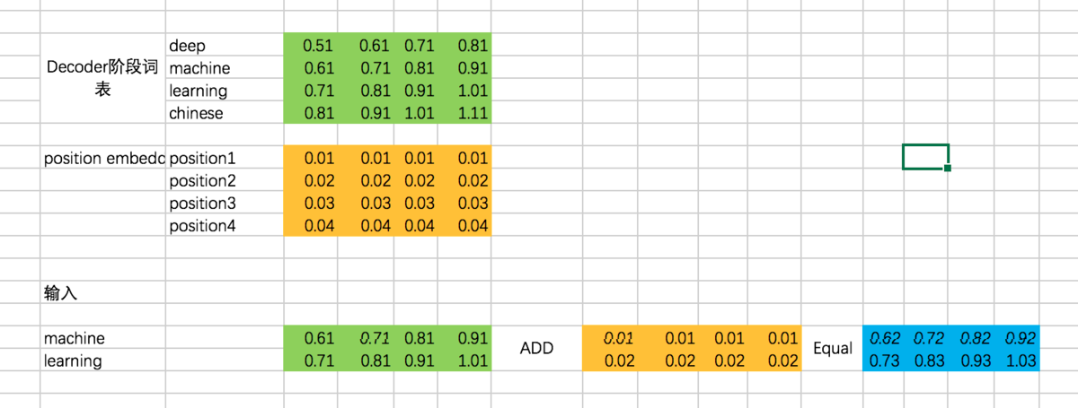
(1) Decoder输入
总体input : [机、器、学、习] -> [ machine、learning]
因此,Decoder阶段的输入是:[ machine、learning]
代码:
english_embedding = tf.constant([[0.51,0.61,0.71,0.81],
                         [0.61,0.71,0.81,0.91],
                         [0.71,0.81,0.91,1.01],
                         [0.81,0.91,1.01,1.11]],dtype=tf.float32)


position_encoding = tf.constant([[0.01,0.01,0.01,0.01],
                         [0.02,0.02,0.02,0.02],
                         [0.03,0.03,0.03,0.03],
                         [0.04,0.04,0.04,0.04]],dtype=tf.float32)

decoder_input = tf.constant([[1,2],[2,1]],dtype=tf.int32)

with tf.variable_scope("decoder_input"):
    decoder_embedding_input = tf.nn.embedding_lookup(english_embedding,decoder_input)
    decoder_embedding_input = decoder_embedding_input + position_encoding[0:tf.shape(decoder_embedding_input)[1]]
(2) masked multi-head self attention
这个过程和multi-head self attention基本一致,只不过对于decoder来说,得到每个阶段的输出时,我们是看不到后面的信息的。举个例子,我们的第一条输入是:[机、器、学、习] -> [ machine、learning] ,decoder阶段两次的输入分别是machine和learning,在输入machine时,我们是看不到learning的信息的,因此在计算attention的权重的时候,machine和learning的权重是没有的。我们还是先通过excel来演示一下,再通过代码来理解:
计算Attention的权重矩阵是:
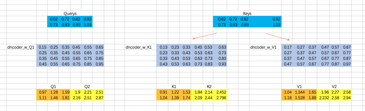
仍然以两个Head为例,计算Q、K、V:
分别计算两个Head的attention map
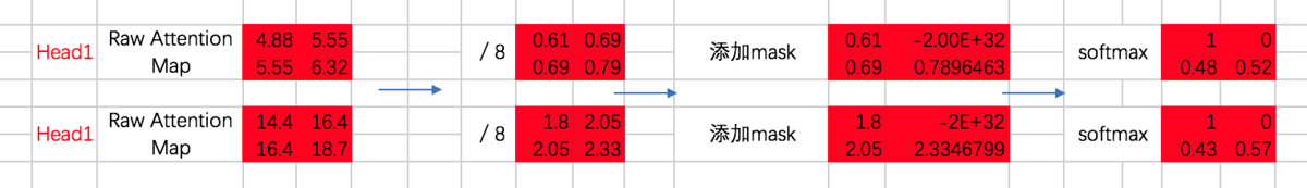
咱们先来实现这部分的代码,masked attention map的计算过程:
前两步和encoder一样,只是得到attention map [ Q*KT / sqrt(dk) ]之后加上masked.然后再softmax ,最后与V相乘.
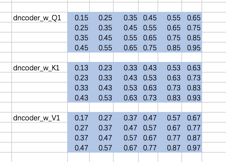
- 先定义下权重矩阵,同encoder一样,定义成常数:
w_Q_decoder_sa = tf.constant([[0.15,0.25,0.35,0.45,0.55,0.65],
                   [0.25,0.35,0.45,0.55,0.65,0.75],
                   [0.35,0.45,0.55,0.65,0.75,0.85],
                   [0.45,0.55,0.65,0.75,0.85,0.95]],dtype=tf.float32)

w_K_decoder_sa = tf.constant([[0.13,0.23,0.33,0.43,0.53,0.63],
                   [0.23,0.33,0.43,0.53,0.63,0.73],
                   [0.33,0.43,0.53,0.63,0.73,0.83],
                   [0.43,0.53,0.63,0.73,0.83,0.93]],dtype=tf.float32)

w_V_decoder_sa = tf.constant([[0.17,0.27,0.37,0.47,0.57,0.67],
                   [0.27,0.37,0.47,0.57,0.67,0.77],
                   [0.37,0.47,0.57,0.67,0.77,0.87],
                   [0.47,0.57,0.67,0.77,0.87,0.97]],dtype=tf.float32)
- 随后,计算添加mask之前的attention map:
with tf.variable_scope("decoder_sa_block"):
    decoder_Q = tf.matmul(tf.reshape(decoder_embedding_input,(-1,tf.shape(decoder_embedding_input)[2])),w_Q_decoder_sa)
    decoder_K = tf.matmul(tf.reshape(decoder_embedding_input,(-1,tf.shape(decoder_embedding_input)[2])),w_K_decoder_sa)
    decoder_V = tf.matmul(tf.reshape(decoder_embedding_input,(-1,tf.shape(decoder_embedding_input)[2])),w_V_decoder_sa)

    decoder_Q = tf.reshape(decoder_Q,(tf.shape(decoder_embedding_input)[0],tf.shape(decoder_embedding_input)[1],-1))
    decoder_K = tf.reshape(decoder_K,(tf.shape(decoder_embedding_input)[0],tf.shape(decoder_embedding_input)[1],-1))
    decoder_V = tf.reshape(decoder_V,(tf.shape(decoder_embedding_input)[0],tf.shape(decoder_embedding_input)[1],-1))

    decoder_Q_split = tf.split(decoder_Q,2,axis=2)
    decoder_K_split = tf.split(decoder_K,2,axis=2)
    decoder_V_split = tf.split(decoder_V,2,axis=2)

    decoder_Q_concat = tf.concat(decoder_Q_split,axis=0)
    decoder_K_concat = tf.concat(decoder_K_split,axis=0)
    decoder_V_concat = tf.concat(decoder_V_split,axis=0)

    decoder_sa_attention_map_raw = tf.matmul(decoder_Q_concat,tf.transpose(decoder_K_concat,[0,2,1]))
    decoder_sa_attention_map = decoder_sa_attention_map_raw / 8
- 随后,对attention map添加mask:
diag_vals = tf.ones_like(decoder_sa_attention_map[0,:,:])
tril = tf.contrib.linalg.LinearOperatorTriL(diag_vals).to_dense()
masks = tf.tile(tf.expand_dims(tril,0),[tf.shape(decoder_sa_attention_map)[0],1,1])
paddings = tf.ones_like(masks) * (-2 ** 32 + 1)
decoder_sa_attention_map = tf.where(tf.equal(masks,0),paddings,decoder_sa_attention_map)
#softmax
decoder_sa_attention_map = tf.nn.softmax(decoder_sa_attention_map)
这里我们首先构造一个全1的矩阵diag_vals,这个矩阵的大小同attention map。随后通过tf.contrib.linalg.LinearOperatorTriL方法把上三角部分变为0,该函数的示意如下:
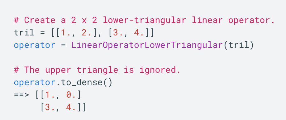
基于这个函数生成的矩阵tril,我们便可以构造对应的mask了。不过需要注意的是,对于我们要加mask的地方,不能赋值为0,而是需要赋值一个很小的数,这里为-2^32 + 1。因为我们后面要做softmax,e^0=1,是一个很大的数啦。
- 补全multi-head attention得到attention map 后面的代码
weightedSumV = tf.matmul(decoder_sa_attention_map,decoder_V_concat)

decoder_outputs_z = tf.concat(tf.split(weightedSumV,2,axis=0),axis=2)

decoder_sa_outputs = tf.matmul(tf.reshape(decoder_outputs_z,(-1,tf.shape(decoder_outputs_z)[2])),w_Z_decoder_sa)

decoder_sa_outputs = tf.reshape(decoder_sa_outputs,(tf.shape(decoder_embedding_input)[0],tf.shape(decoder_embedding_input)[1],-1))


with tf.Session() as sess:
    print(sess.run(decoder_sa_outputs))
(3)encoder-decoder attention
在encoder-decoder attention之间,还有一个Add & Normalize的过程,同样,我们忽略 Normalize,只做Add操作:
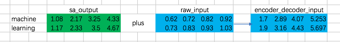
接下来,就是encoder-decoder了,这里跟multi-head attention相同,但是需要注意的一点是,我们这里想要做的是,计算decoder的每个阶段的输入和encoder阶段所有输出的attention,所以Q的计算通过decoder对应的embedding计算,而K和V通过encoder阶段输出的embedding来计算:
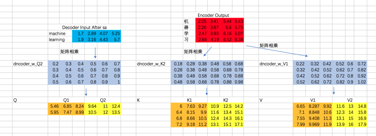
接下来,计算Attention Map,注意,这里attention map的大小为2 * 4的,每一行代表一个decoder的输入,与所有encoder输出之间的attention score。同时,我们不需要添加mask,因为decoder的输入是可以看到所有encoder的输出信息的。得到的attention map结果如下:
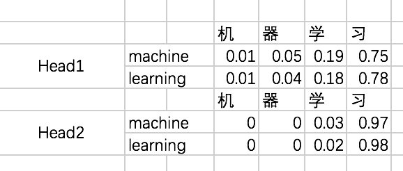
接下来,我们得到整个encoder-decoder阶段的输出为:
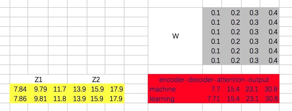
接下来,还有Add & Normalize、Feed Forward Network、Add & Normalize过程,咱们这里就省略了。encoder-decoder代码:
w_Q_decoder_sa2 = tf.constant([[0.2,0.3,0.4,0.5,0.6,0.7],
                   [0.3,0.4,0.5,0.6,0.7,0.8],
                   [0.4,0.5,0.6,0.7,0.8,0.9],
                   [0.5,0.6,0.7,0.8,0.9,1]],dtype=tf.float32)

w_K_decoder_sa2 = tf.constant([[0.18,0.28,0.38,0.48,0.58,0.68],
                   [0.28,0.38,0.48,0.58,0.68,0.78],
                   [0.38,0.48,0.58,0.68,0.78,0.88],
                   [0.48,0.58,0.68,0.78,0.88,0.98]],dtype=tf.float32)

w_V_decoder_sa2 = tf.constant([[0.22,0.32,0.42,0.52,0.62,0.72],
                   [0.32,0.42,0.52,0.62,0.72,0.82],
                   [0.42,0.52,0.62,0.72,0.82,0.92],
                   [0.52,0.62,0.72,0.82,0.92,1.02]],dtype=tf.float32)

w_Z_decoder_sa2 = tf.constant([[0.1,0.2,0.3,0.4],
                   [0.1,0.2,0.3,0.4],
                   [0.1,0.2,0.3,0.4],
                   [0.1,0.2,0.3,0.4],
                   [0.1,0.2,0.3,0.4],
                   [0.1,0.2,0.3,0.4]],dtype=tf.float32)


with tf.variable_scope("decoder_encoder_attention_block"):

    decoder_sa_outputs = decoder_sa_outputs + decoder_embedding_input

    encoder_decoder_Q = tf.matmul(tf.reshape(decoder_sa_outputs,(-1,tf.shape(decoder_sa_outputs)[2])),w_Q_decoder_sa2)
    encoder_decoder_K = tf.matmul(tf.reshape(encoder_outputs,(-1,tf.shape(encoder_outputs)[2])),w_K_decoder_sa2)
    encoder_decoder_V = tf.matmul(tf.reshape(encoder_outputs,(-1,tf.shape(encoder_outputs)[2])),w_V_decoder_sa2)

    encoder_decoder_Q = tf.reshape(encoder_decoder_Q,(tf.shape(decoder_embedding_input)[0],tf.shape(decoder_embedding_input)[1],-1))
    encoder_decoder_K = tf.reshape(encoder_decoder_K,(tf.shape(encoder_outputs)[0],tf.shape(encoder_outputs)[1],-1))
    encoder_decoder_V = tf.reshape(encoder_decoder_V,(tf.shape(encoder_outputs)[0],tf.shape(encoder_outputs)[1],-1))

    encoder_decoder_Q_split = tf.split(encoder_decoder_Q,2,axis=2)
    encoder_decoder_K_split = tf.split(encoder_decoder_K,2,axis=2)
    encoder_decoder_V_split = tf.split(encoder_decoder_V,2,axis=2)

    encoder_decoder_Q_concat = tf.concat(encoder_decoder_Q_split,axis=0)
    encoder_decoder_K_concat = tf.concat(encoder_decoder_K_split,axis=0)
    encoder_decoder_V_concat = tf.concat(encoder_decoder_V_split,axis=0)
    ##注意,不用mask
    encoder_decoder_attention_map_raw = tf.matmul(encoder_decoder_Q_concat,tf.transpose(encoder_decoder_K_concat,[0,2,1]))
    encoder_decoder_attention_map = encoder_decoder_attention_map_raw / 8

    encoder_decoder_attention_map = tf.nn.softmax(encoder_decoder_attention_map)

    weightedSumV = tf.matmul(encoder_decoder_attention_map,encoder_decoder_V_concat)

    encoder_decoder_outputs_z = tf.concat(tf.split(weightedSumV,2,axis=0),axis=2)

    encoder_decoder_outputs = tf.matmul(tf.reshape(encoder_decoder_outputs_z,(-1,tf.shape(encoder_decoder_outputs_z)[2])),w_Z_decoder_sa2)

    encoder_decoder_attention_outputs = tf.reshape(encoder_decoder_outputs,(tf.shape(decoder_embedding_input)[0],tf.shape(decoder_embedding_input)[1],-1))

    encoder_decoder_attention_outputs = encoder_decoder_attention_outputs + decoder_sa_outputs

    # todo :add BN
    W_f = tf.constant([[0.2,0.3,0.5,0.4],
                       [0.2,0.3,0.5,0.4],
                       [0.2,0.3,0.5,0.4],
                       [0.2,0.3,0.5,0.4]])

    decoder_ffn_outputs = tf.matmul(tf.reshape(encoder_decoder_attention_outputs,(-1,tf.shape(encoder_decoder_attention_outputs)[2])),W_f)
    decoder_ffn_outputs = tf.reshape(decoder_ffn_outputs,(tf.shape(encoder_decoder_attention_outputs)[0],tf.shape(encoder_decoder_attention_outputs)[1],-1))

    decoder_outputs = decoder_ffn_outputs + encoder_decoder_attention_outputs
    # todo :add BN

with tf.Session() as sess:
    print(sess.run(decoder_outputs))
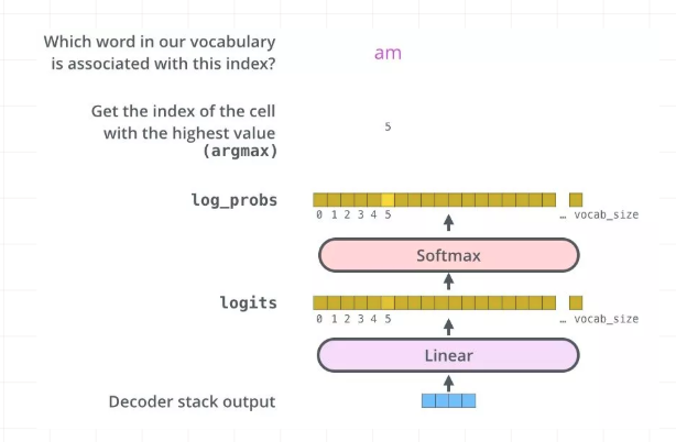
(4)全连接层及最终输出
最后的全连接层很简单了,对于decoder阶段的输出,通过全连接层和softmax之后,最终得到选择每个单词的概率,并计算交叉熵损失:
代码:
W_final = tf.constant([[0.2,0.3,0.5,0.4],
                       [0.2,0.3,0.5,0.4],
                       [0.2,0.3,0.5,0.4],
                       [0.2,0.3,0.5,0.4]])

logits = tf.matmul(tf.reshape(decoder_outputs,(-1,tf.shape(decoder_outputs)[2])),W_final)
logits = tf.reshape(logits,(tf.shape(decoder_outputs)[0],tf.shape(decoder_outputs)[1],-1))


logits = tf.nn.softmax(logits)

y = tf.one_hot(decoder_input,depth=4)

loss = tf.nn.softmax_cross_entropy_with_logits(logits=logits,labels=y)

train_op = tf.train.AdamOptimizer(learning_rate=0.0001).minimize(loss)
参考:
https://www.jianshu.com/p/3f2d4bc126e6
https://www.leiphone.com/news/201709/8tDpwklrKubaecTa.html
https://www.cnblogs.com/hellojamest/p/11128799.html
https://blog.csdn.net/longxinchen_ml/article/details/86533005
https://www.imooc.com/article/67493
李宏毅老师的课程
NLP 学习:http://www.shuang0420.com/categories/NLP/page/9/