多层神经网络与应用—MNIST手写数字识别（一）

一、单隐藏层神经网络构建与应用

主要内容：

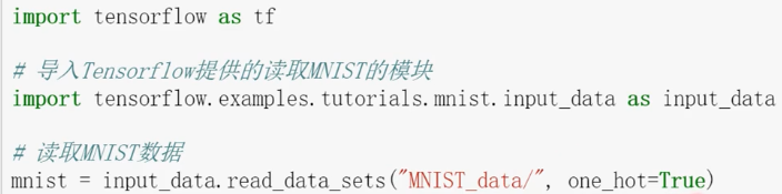
　　1.1载入数据

　　1.2建立模型

　　1.3训练模型

　　1.4评估模型

　　1.5应用模型

1.1载入数据

 1.2建立模型

1.2.1构建输入层

#定义标签数据占位符
x= tf.placeholder(tf.float32, [None, 784], name='X') #图片大小28*28
y= tf.placeholder(tf.float32, [None, 10], name='Y')

1.2.2构建隐藏层

H1_NN=256  #自定义隐藏层神经元数量
W1 = tf.Variable(tf.random_normal([784,H1_NN])) #全连接x1,x2...
b1 = tf.Variable(tf.zeros([H1_NN]))    #偏置项
Y1 = tf.nn.relu(tf.matmul(x,W1)+b1)

1.2.3构建输出层

W2 = tf.Variable(tf.random_normal([H1_NN,10]))
b2 = tf.Variable(tf.zeros([10]))
forward = tf.matmul(Y1, W2) + b2
pred=tf.nn.softmax(forward)  #多分类预测结果

1.3训练模型

1.3.1定义损失函数、设置训练参数、选择优化器、定义准确率

loss_function = tf.reduce_mean(-tf.reduce_sum(y*tf.log(pred),reduction_indices=1))   #定义交叉熵损失函数

#设置训练参数
train_epochs = 40   #训练轮数
batch_size=50      #单次训练样本数（批次大小)
total_batch= int(mnist.train.num_examples/batch_size)#一轮训练有多少批次
display_step=1     #显示粒度
learning_rate=0.01   #学习率

#选择优化器
optimizer = tf.train.AdamOptimizer(learning_rate).minimize(loss_function)

#定义准确率
correct_prediction = tf.equal(tf.argmax(y,1),tf.argmax(pred,1))
accuracy = tf.reduce_mean(tf.cast(correct_prediction,tf.float32))#准确率，将布尔值转化为浮点数，并计算平均值

1.3.2训练过程

#记录训练开始时间
startTime = time()

sess = tf.Session()
sess.run(tf.global_variables_initializer())

for epoch in range(train_epochs):
    for batch in range(total_batch):
          xs, ys = mnist.train.next_batch(batch_size)  # 读取批次数据
          sess.run(optimizer,feed_dict={x:xs,y:ys})   # 执行批次训练
    #total_batch个批次训练完成后，使用验证数据计算课差与准确率；验证集没有分批
    loss,acc = sess.run([loss_function,accuracy],feed_dict={x:mnist.validation.images,y:mnist.validation.labels})
    #打印训练过程中的详细信息
    if (epoch+1) % display_step == 0:
        print("Train Epoch:",'%02d' %(epoch+1),"Loss=","{:.9f}".format(loss),"Accuracy=","{:.4f}".format(acc))

duration = time()-startTime  #显示运行总时间
print("Train Finished takes:","{:.2f}".format(duration))

运行结果为：

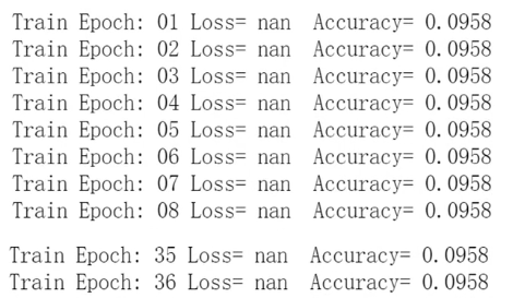
 分析原因，定义交叉熵损失函数时，有一个log项，log(0)引起的数据不稳定

# loss_function = tf.reduce_mean(-tf.reduce_sum(y*tf.log(pred),reduction_indices=1))   #定义交叉熵损失函数
#TensorFlow提供了softmax_cross_entropy_with_logits函数，用于避免因为log(0)值为NaN造成的数据不稳定
loss_function = tf.reduce_mean(tf.nn.softmax_cross_entropy_with_logits(logits=forward,labels=y))  #注意第一个参数是不做Softmax的前向计算结果

修改后，运行结果为：

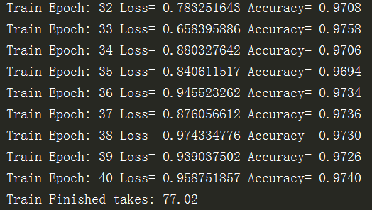
从上述打印结果可以看出包含256个神经元的单隐层神经网络的分类性能比仅包含一个网络更优。

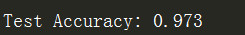
1.4评估模型

#使用测试集评估模型
accu_test = sess.run(accuracy,feed_dict={x:mnist.test.images,y:mnist.test.labels})
print("Test Accuracy:",accu_test)

1.5应用模型

1.5.1进行预测

#由于pred预测结果是one-hot编码格式，所以需要转换为0-9数字
prediction_result = sess.run(tf.argmax(pred,1),feed_dict={x:mnist.test.images})
print(prediction_result[0:10])  #查看预测结果中的前10项

 1.5.2找出预测错误

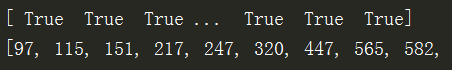
compare_lists = prediction_result==np.argmax(mnist.test.labels,1)
print(compare_lists)

err_lists=[i for i in range(len(compare_lists)) if compare_lists[i]==False]
print(err_lists, len(err_lists))  #最后一项即为多少个预测错了

     ........... 

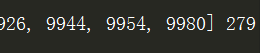
 可见一共有279个预测错误，但这样返回预测错误的下标不够直观，接下来进行修改。

修改一：

#定义一个输出错误分类的函数
def print_predict_errs(labels, prediction):   #标签列表，预测值列表
    count = 0
    compare_lists =(prediction==np.argmax(labels,1))
    err_lists = [i for i in range(len(compare_lists)) if compare_lists [i]==False]
    for x in err_lists:
        print("index="+str(x) + "标签值=",np.argmax(labels[x]),"预测值=",prediction[x])
        count += 1
    print("总计:"+str(count))

print_predict_errs(labels=mnist.test.labels,prediction=prediction_result)

运行结果：

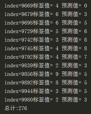
 以文本显示，仍然不够直观，进一步修改。

修改二（+可视化）：

对https://www.cnblogs.com/HuangYJ/p/11642475.html中6.1节可视化函数修改，以便只显示预测错误的样本

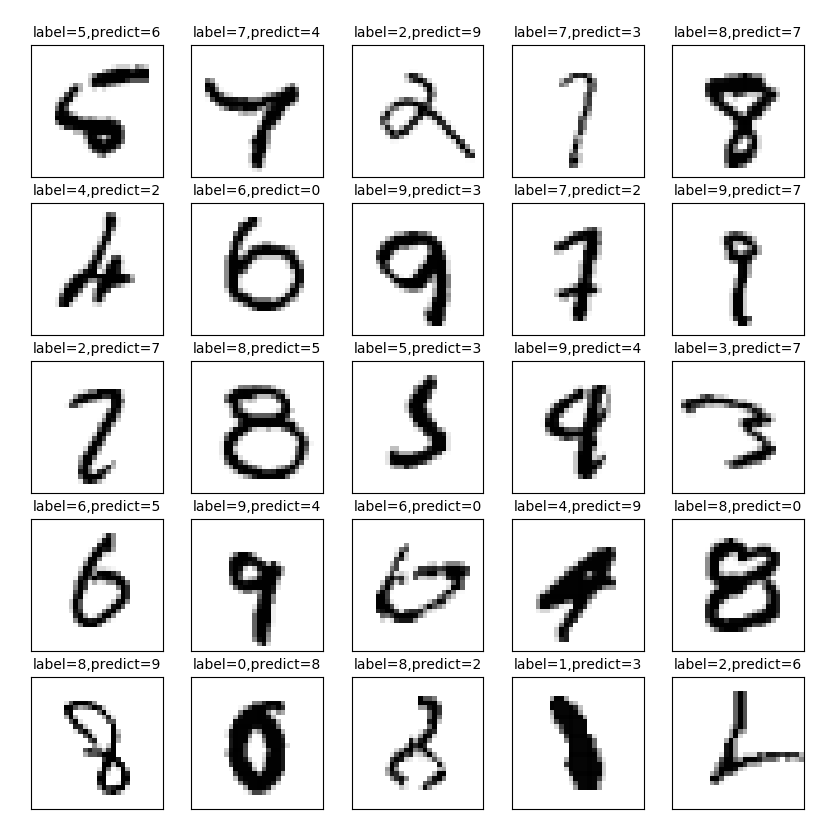
#可视化
def plot_images_labels_prediction(images,labels,prediction,num=10):   #图像列表，标签列表，预测值列表，从第index个开始显示 ， 缺省一次显示10幅
    j = 0
    fig = plt.gcf() #获取当前图表，get current figure
    fig.set_size_inches(10,12)  #1英寸等于2.54cm

    compare_lists = prediction_result == np.argmax(mnist.test.labels, 1)
    err_lists = [i for i in range(len(compare_lists)) if compare_lists[i] == False]

    if num > 25:
        num = 25  #最多显示25个子图

    for i in range(0, num):
        ax = plt.subplot(5,5,i+1)  #获取当前要处理的子图
        ax.imshow(np.reshape(images[err_lists[j]], (28, 28)),cmap='binary')  # 显示第index个图像
        title = "label=" + str(np.argmax(labels[err_lists[j]]))# 构建该图上要显示的
        if len(prediction)>0:
            title += ",predict="+ str(prediction[err_lists[j]])
        ax.set_title(title, fontsize=10)  #显示图上title信息
        ax.set_xticks([])  #不显示坐标轴
        ax.set_yticks([])
        j += 1
    plt.show()

plot_images_labels_prediction(mnist.test.images,mnist.test.labels,prediction_result,25)  #最多显示25张

显示前25个预测错误的样本，预测结果为：

全部代码为：

#Created by:Huang
#Time:2019/10/15 0015.

import tensorflow as tf
import tensorflow.examples.tutorials.mnist.input_data as input_data
import matplotlib.pyplot as plt
import numpy as np
from time import time

mnist = input_data.read_data_sets("MNIST_data/",one_hot=True)

#定义标签数据占位符
x= tf.placeholder(tf.float32, [None, 784], name='X') #图片大小28*28
y= tf.placeholder(tf.float32, [None, 10], name='Y')

#隐藏层
H1_NN=256  #自定义隐藏层神经元数量
W1 = tf.Variable(tf.random_normal([784,H1_NN])) #全连接x1,x2...
b1 = tf.Variable(tf.zeros([H1_NN]))    #偏置项
Y1 = tf.nn.relu(tf.matmul(x,W1)+b1)

#输出层
W2 = tf.Variable(tf.random_normal([H1_NN,10]))
b2 = tf.Variable(tf.zeros([10]))
forward = tf.matmul(Y1, W2) + b2
pred=tf.nn.softmax(forward)  #多分类预测结果


# loss_function = tf.reduce_mean(-tf.reduce_sum(y*tf.log(pred),reduction_indices=1))   #定义交叉熵损失函数
#TensorFlow提供了softmax_cross_entropy_with_logits函数，用于避免因为log(0)值为NaN造成的数据不稳定
loss_function = tf.reduce_mean(tf.nn.softmax_cross_entropy_with_logits(logits=forward,labels=y))  #注意第一个参数是不做Softmax的前向计算结果


#设置训练参数
train_epochs = 40   #训练轮数
batch_size=50      #单次训练样本数（批次大小)
total_batch= int(mnist.train.num_examples/batch_size)#一轮训练有多少批次
display_step=1     #显示粒度
learning_rate=0.01   #学习率

#选择优化器
optimizer = tf.train.AdamOptimizer(learning_rate).minimize(loss_function)

#定义准确率
correct_prediction = tf.equal(tf.argmax(y,1),tf.argmax(pred,1))
accuracy = tf.reduce_mean(tf.cast(correct_prediction,tf.float32))#准确率，将布尔值转化为浮点数，并计算平均值

#记录训练开始时间
startTime = time()

sess = tf.Session()
sess.run(tf.global_variables_initializer())

for epoch in range(train_epochs):
    for batch in range(total_batch):
          xs, ys = mnist.train.next_batch(batch_size)  # 读取批次数据
          sess.run(optimizer,feed_dict={x:xs,y:ys})   # 执行批次训练
    #total_batch个批次训练完成后，使用验证数据计算课差与准确率；验证集没有分批
    loss,acc = sess.run([loss_function,accuracy],feed_dict={x:mnist.validation.images,y:mnist.validation.labels})
    #打印训练过程中的详细信息
    if (epoch+1) % display_step == 0:
        print("Train Epoch:",'%02d' %(epoch+1),"Loss=","{:.9f}".format(loss),"Accuracy=","{:.4f}".format(acc))

duration = time()-startTime  #显示运行总时间
print("Train Finished takes:","{:.2f}".format(duration))

#使用测试集评估模型
accu_test = sess.run(accuracy,feed_dict={x:mnist.test.images,y:mnist.test.labels})
print("Test Accuracy:",accu_test)

#模型预测
#由于pred预测结果是one-hot编码格式，所以需要转换为0-9数字
prediction_result = sess.run(tf.argmax(pred,1),feed_dict={x:mnist.test.images})
print(prediction_result[0:10])  #查看预测结果中的前10项

# #找出预测错误
# compare_lists = prediction_result==np.argmax(mnist.test.labels,1)
# print(compare_lists)
#
# err_lists=[i for i in range(len(compare_lists)) if compare_lists[i]==False]
# print(err_lists, len(err_lists))  #最后一项即为多少个预测错了

#定义一个输出错误分类的函数
# def print_predict_errs(labels, prediction):   #标签列表，预测值列表
#     count = 0
#     compare_lists =(prediction==np.argmax(labels,1))
#     err_lists = [i for i in range(len(compare_lists)) if compare_lists [i]==False]
#     for x in err_lists:
#         print("index="+str(x) + "标签值=",np.argmax(labels[x]),"预测值=",prediction[x])
#         count += 1
#     print("总计:"+str(count))

# print_predict_errs(labels=mnist.test.labels,prediction=prediction_result)


#可视化
def plot_images_labels_prediction(images,labels,prediction,num=10):   #图像列表，标签列表，预测值列表，从第index个开始显示 ， 缺省一次显示10幅
    j = 0
    fig = plt.gcf() #获取当前图表，get current figure
    fig.set_size_inches(10,12)  #1英寸等于2.54cm

    compare_lists = prediction_result == np.argmax(mnist.test.labels, 1)
    err_lists = [i for i in range(len(compare_lists)) if compare_lists[i] == False]

    if num > 25:
        num = 25  #最多显示25个子图

    for i in range(0, num):
        ax = plt.subplot(5,5,i+1)  #获取当前要处理的子图
        ax.imshow(np.reshape(images[err_lists[j]], (28, 28)),cmap='binary')  # 显示第index个图像
        title = "label=" + str(np.argmax(labels[err_lists[j]]))# 构建该图上要显示的
        if len(prediction)>0:
            title += ",predict="+ str(prediction[err_lists[j]])
        ax.set_title(title, fontsize=10)  #显示图上title信息
        ax.set_xticks([])  #不显示坐标轴
        ax.set_yticks([])
        j += 1
    plt.show()

plot_images_labels_prediction(mnist.test.images,mnist.test.labels,prediction_result,25)  #最多显示25张