R语言学习笔记（十）：重抽样与自助法

#置换实验 Coin包
install.packages(c("coin"))

#lmPerm包
install.packages("lmPerm")


#独立两样本和K样本检验
library(coin)
score<-c(40,57,45,55,58,57,64,55,62,65)
treatment<-factor(c(rep("A",5),rep("B",5)))
mydata<-data.frame(treatment,score)
t.test(score~treatment,data=mydata,var.equal=TRUE)

Two Sample t-test

data: score by treatment
t = -2.345, df = 8, p-value = 0.04705
alternative hypothesis: true difference in means is not equal to 0
95 percent confidence interval:
-19.0405455 -0.1594545
sample estimates:
mean in group A mean in group B
51.0 60.6

#置换T检验
library(coin)
oneway_test(score~treatment,data=mydata,distribution="exact")

Exact Two-Sample Fisher-Pitman Permutation Test

data: score by treatment (A, B)
Z = -1.9147, p-value = 0.07143
alternative hypothesis: true mu is not equal to 0

结果显著：P<0.05

结果不显著：P>0.05

上面这两个测试中所得的P值相差比较大，并且样本容易比较小，所以置换T检验更有说服力，因此我们认为改组样本得到的结果不显著P>0.05

#Wilcox.test
library(MASS)
UScrime<-transform(UScrime,So=factor(So))
wilcox_test(Prob~So,data=UScrime,distribution="exact")

Exact Wilcoxon-Mann-Whitney Test

data: Prob by So (0, 1)
Z = -3.7493, p-value = 8.488e-05
alternative hypothesis: true mu is not equal to 0

wilcox.test(Prob~So,data=UScrime,distribution="exact")

Wilcoxon rank sum test

data: Prob by So
W = 81, p-value = 8.488e-05
alternative hypothesis: true location shift is not equal to 0

#chisq_Test
library(coin)
library(vcd)
Arthritis<-transform(Arthritis,Improved=as.factor(as.numeric(Improved)))
set.seed(1234)
chisq_test(Treatment~Improved,data=Arthritis,distribution=approximate(B=9999))

Approximative Pearson Chi-Squared Test

data: Treatment by Improved (1, 2, 3)
chi-squared = 13.055, p-value = 0.0018

#spearman.test 数值变量间的独立性
states<-as.data.frame(state.x77)
set.seed(1234)
spearman_test(Illiteracy~Murder,data=states,distribution=approximate(B=9999))

Approximative Spearman Correlation Test

data: Illiteracy by Murder
Z = 4.7065, p-value < 2.2e-16
alternative hypothesis: true rho is not equal to 0

#两样本和K样本相关性检验
library(coin)
library(MASS)
wilcoxsign_test(U1~U2,data=UScrime,distribution="exact")

Exact Wilcoxon-Pratt Signed-Rank Test

data: y by x (pos, neg)
stratified by block
Z = 5.9691, p-value = 1.421e-14
alternative hypothesis: true mu is not equal to 0

#lmPerm包的置换检验
library(lmPerm)

#简单线性回归置换
set.seed(1234)
fit<-lmp(weight~height,data=women,perm="Prob")
summary(fit)

Call:
lmp(formula = weight ~ height, data = women, perm = "Prob")

Residuals:
Min 1Q Median 3Q Max
-1.7333 -1.1333 -0.3833 0.7417 3.1167

Coefficients:
Estimate Iter Pr(Prob)
height 3.45 5000 <2e-16 ***
---
Signif. codes: 0 ‘***’ 0.001 ‘**’ 0.01 ‘*’ 0.05 ‘.’ 0.1 ‘ ’ 1

Residual standard error: 1.525 on 13 degrees of freedom
Multiple R-Squared: 0.991, Adjusted R-squared: 0.9903
F-statistic: 1433 on 1 and 13 DF, p-value: 1.091e-14

#多项式回归的置换检验
set.seed(1234)
fit<-lmp(weight~height+I(height^2),data=women,perm="Prob")
summary(fit)

Call:
lmp(formula = weight ~ height + I(height^2), data = women, perm = "Prob")

Residuals:
Min 1Q Median 3Q Max
-0.509405 -0.296105 -0.009405 0.286151 0.597059

Coefficients:
Estimate Iter Pr(Prob)
height -7.34832 5000 <2e-16 ***
I(height^2) 0.08306 5000 <2e-16 ***
---
Signif. codes: 0 ‘***’ 0.001 ‘**’ 0.01 ‘*’ 0.05 ‘.’ 0.1 ‘ ’ 1

Residual standard error: 0.3841 on 12 degrees of freedom
Multiple R-Squared: 0.9995, Adjusted R-squared: 0.9994
F-statistic: 1.139e+04 on 2 and 12 DF, p-value: < 2.2e-16

#多元回归
library(lmPerm)
set.seed(1234)
states<-as.data.frame(state.x77)
fit<-lmp(Murder~Population+Illiteracy+Income+Frost,data=states,perm="Prob")
summary(fit)

Call:
lmp(formula = Murder ~ Population + Illiteracy + Income + Frost,
data = states, perm = "Prob")

Residuals:
Min 1Q Median 3Q Max
-4.79597 -1.64946 -0.08112 1.48150 7.62104

Coefficients:
Estimate Iter Pr(Prob)
Population 2.237e-04 51 1.0000
Illiteracy 4.143e+00 5000 0.0004 ***
Income 6.442e-05 51 1.0000
Frost 5.813e-04 51 0.8627
---
Signif. codes: 0 ‘***’ 0.001 ‘**’ 0.01 ‘*’ 0.05 ‘.’ 0.1 ‘ ’ 1

Residual standard error: 2.535 on 45 degrees of freedom
Multiple R-Squared: 0.567, Adjusted R-squared: 0.5285
F-statistic: 14.73 on 4 and 45 DF, p-value: 9.133e-08

#单因素方差分析和协方差分析
library(lmPerm)
library(multcomp)
set.seed(1234)
fit<-aovp(response~trt,data=cholesterol,perm="Prob")
anova(fit)

Analysis of Variance Table

Response: response
Df R Sum Sq R Mean Sq Iter Pr(Prob)
trt 4 1351.37 337.84 5000 < 2.2e-16 ***
Residuals 45 468.75 10.42
---
Signif. codes: 0 ‘***’ 0.001 ‘**’ 0.01 ‘*’ 0.05 ‘.’ 0.1 ‘ ’ 1

#双因素方差分析
library(lmPerm)
set.seed(1234)
fit<-aovp(len~supp*dose,data=ToothGrowth,perm="Prob")
anova(fit)

Analysis of Variance Table

Response: len
Df R Sum Sq R Mean Sq Iter Pr(Prob)
supp 1 205.35 205.35 5000 < 2e-16 ***
dose 1 2224.30 2224.30 5000 < 2e-16 ***
supp:dose 1 88.92 88.92 2032 0.04724 *
Residuals 56 933.63 16.67
---
Signif. codes: 0 ‘***’ 0.001 ‘**’ 0.01 ‘*’ 0.05 ‘.’ 0.1 ‘ ’ 1

#自助法
library(boot)
set.seed(1234)
rsq<-function(formula,data,indices){
  d<-data[indices,]
  fit<-lm(formula,data=d)
  return(summary(fit)$r.square)
  
}


results<-boot(data=mtcars,statistic=rsq,R=1000,formula=mpg~wt+disp)
print(results)

boot.ci(results,type=c("perc","bca"))

BOOTSTRAP CONFIDENCE INTERVAL CALCULATIONS
Based on 1000 bootstrap replicates

CALL :
boot.ci(boot.out = results, type = c("perc", "bca"))

Intervals :
Level Percentile BCa
95% ( 0.6838, 0.8833 ) ( 0.6344, 0.8549 )
Calculations and Intervals on Original Scale
Some BCa intervals may be unstable

#多个统计量的自助法
bs<-function(formula,data,indices){
  d<-data[indices,]
  fit<-lm(formula,data=d)
  return(coef(fit))
  
}

library(boot)
set.seed(1234)
results<-boot(data=mtcars,statistic=bs,R=1000,formula=mpg~wt+disp)
print(results)


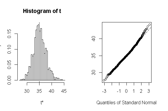
plot(results,index=1)