一、逻辑回归的介绍
logistic回归又称logistic回归分析,是一种广义的线性回归分析模型,常用于数据挖掘,疾病自动诊断,经济预测等领域。例如,探讨引发疾病的危险因素,并根据危险因素预测疾病发生的概率等。以胃癌病情分析为例,选择两组人群,一组是胃癌组,一组是非胃癌组,两组人群必定具有不同的体征与生活方式等。因此因变量就为是否胃癌,值为“是”或“否”,自变量就可以包括很多了,如年龄、性别、饮食习惯、幽门螺杆菌感染等。自变量既可以是连续的,也可以是分类的。然后通过logistic回归分析,可以得到自变量的权重,从而可以大致了解到底哪些因素是胃癌的危险因素。同时根据该权值可以根据危险因素预测一个人患癌症的可能性。
二、逻辑回归的原理和实现
逻辑回归的算法原理和线性回归的算法步骤大致相同,只是预测函数H和权值更新规则不同。逻辑回归算法在这里应用于多分类,由于MNIST的数据集是共有十类的手写数字图片,所以应该使用十个分类器模型,分别求出每类最好的权值向量,并将其应用到预测函数中,预测函数值相当于概率,使得预测函数值最大对应的类就是所预测的类。
三、数据集介绍
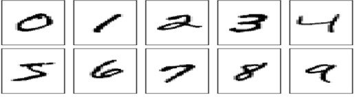
MNIST数据集,MNIST 数据集来自美国国家标准与技术研究所,National Institute of Standards and Technology (NIST). 训练集 (training set) 由来自 250 个不同人手写的数字构成, 其中 50% 是高中学生, 50% 来自人口普查局 (the Census Bureau) 的工作人员. 测试集(test set) 也是同样比例的手写数字数据。训练数据集共有60000张图片和相应的标签,测试数据集共有10000张图片和相应的标签,并且每个图片都有28*28个像素。图1大致展示了数据集中的手写图片。
四、逻辑回归的代码和结果
代码:
from numpy import *
import operator
import os
import numpy as np
import time
from scipy.special import expit
import matplotlib.pyplot as plt
from matplotlib import cm
from os import listdir
from mpl_toolkits.mplot3d import Axes3D
import struct
import math
#读取图片
def read_image(file_name):
    #先用二进制方式把文件都读进来
    file_handle=open(file_name,"rb")  #以二进制打开文档
    file_content=file_handle.read()   #读取到缓冲区中
    offset=0
    head = struct.unpack_from('>IIII', file_content, offset)  # 取前4个整数,返回一个元组
    offset += struct.calcsize('>IIII')
    imgNum = head[1]  #图片数
    rows = head[2]   #宽度
    cols = head[3]  #高度

    images=np.empty((imgNum , 784))#empty,是它所常见的数组内的所有元素均为空,没有实际意义,它是创建数组最快的方法
    image_size=rows*cols#单个图片的大小
    fmt='>' + str(image_size) + 'B'#单个图片的format

    for i in range(imgNum):
        images[i] = np.array(struct.unpack_from(fmt, file_content, offset))
        # images[i] = np.array(struct.unpack_from(fmt, file_content, offset)).reshape((rows, cols))
        offset += struct.calcsize(fmt)
    return images

#读取标签
def read_label(file_name):
    file_handle = open(file_name, "rb")  # 以二进制打开文档
    file_content = file_handle.read()  # 读取到缓冲区中

    head = struct.unpack_from('>II', file_content, 0)  # 取前2个整数,返回一个元组
    offset = struct.calcsize('>II')

    labelNum = head[1]  # label数
    # print(labelNum)
    bitsString = '>' + str(labelNum) + 'B'  # fmt格式:'>47040000B'
    label = struct.unpack_from(bitsString, file_content, offset)  # 取data数据,返回一个元组
    return np.array(label)

def loadDataSet():
    train_x_filename="train-images-idx3-ubyte"
    train_y_filename="train-labels-idx1-ubyte"
    test_x_filename="t10k-images-idx3-ubyte"
    test_y_filename="t10k-labels-idx1-ubyte"
    train_x=read_image(train_x_filename)
    train_y=read_label(train_y_filename)
    test_x=read_image(test_x_filename)
    test_y=read_label(test_y_filename)

    # # # #调试的时候让速度快点,就先减少数据集大小
    # train_x=train_x[0:1000,:]
    # train_y=train_y[0:1000]
    # test_x=test_x[0:500,:]
    # test_y=test_y[0:500]

    return train_x, test_x, train_y, test_y

def sigmoid(inX):
    return 1.0/(1+exp(-inX))

def classifyVector(inX,weights):#这里的inX相当于test_data,以回归系数和特征向量作为输入来计算对应的sigmoid
    prob=sigmoid(sum(inX*weights))
    if prob>0.5:return 1.0
    else: return 0.0
# train_model(train_x, train_y, theta, learning_rate, iteration,numClass)
def train_model(train_x,train_y,theta,learning_rate,iterationNum,numClass):#theta是n+1行的列向量
    m=train_x.shape[0]
    n=train_x.shape[1]
    train_x=np.insert(train_x,0,values=1,axis=1)
    J_theta = np.zeros((iterationNum,numClass))

    for k in range(numClass):
        # print(k)
        real_y=np.zeros((m,1))
        index=train_y==k#index中存放的是train_y中等于0的索引
        real_y[index]=1#在real_y中修改相应的index对应的值为1,先分类0和非0

        for j in range(iterationNum):
            # print(j)
            temp_theta = theta[:,k].reshape((785,1))
            #h_theta=expit(np.dot(train_x,theta[:,k]))#是m*1的矩阵(列向量),这是概率
            h_theta = expit(np.dot(train_x, temp_theta)).reshape((60000,1))
            #这里的一个问题,将train_y变成0或者1
            J_theta[j,k] = (np.dot(np.log(h_theta).T,real_y)+np.dot((1-real_y).T,np.log(1-h_theta))) / (-m)
            temp_theta = temp_theta + learning_rate*np.dot(train_x.T,(real_y-h_theta))

        #theta[:,k] =learning_rate*np.dot(train_x.T,(real_y-h_theta))
            theta[:, k] = temp_theta.reshape((785,))

    return theta#返回的theta是n*numClass矩阵

def predict(test_x,test_y,theta,numClass):#这里的theta是学习得来的最好的theta,是n*numClass的矩阵
    errorCount=0
    test_x = np.insert(test_x, 0, values=1, axis=1)
    m = test_x.shape[0]


    h_theta=expit(np.dot(test_x,theta))#h_theta是m*numClass的矩阵,因为test_x是m*n,theta是n*numClass
    h_theta_max = h_theta.max(axis=1)  # 获得每行的最大值,h_theta_max是m*1的矩阵,列向量
    h_theta_max_postion=h_theta.argmax(axis=1)#获得每行的最大值的label
    for i in range(m):
        if test_y[i]!=h_theta_max_postion[i]:
            errorCount+=1

    error_rate = float(errorCount) / m
    print("error_rate", error_rate)
    return error_rate

def mulitPredict(test_x,test_y,theta,iteration):
    numPredict=10
    errorSum=0
    for k in range(numPredict):
        errorSum+=predict(test_x,test_y,theta,iteration)
    print("after %d iterations the average error rate is:%f" % (numPredict, errorSum / float(numPredict)))

if __name__=='__main__':
    print("Start reading data...")
    time1=time.time()
    train_x, test_x, train_y, test_y = loadDataSet()
    time2=time.time()
    print("read data cost",time2-time1,"second")

    numClass=10
    iteration = 1
    learning_rate = 0.001
    n=test_x.shape[1]+1

    theta=np.zeros((n,numClass))# theta=np.random.rand(n,1)#随机构造n*numClass的矩阵,因为有numClass个分类器,所以应该返回的是numClass个列向量(n*1)

    print("Start training data...")
    theta_new = train_model(train_x, train_y, theta, learning_rate, iteration,numClass)
    time3 = time.time()
    print("train data cost", time3 - time2, "second")

    print("Start predicting data...")
    predict(test_x, test_y, theta_new,iteration)
    time4=time.time()
    print("predict data cost",time4-time3,"second")
结果截图:
逻辑回归分类MNIST数据集的实验
该实验中用到的参数学习率是0.001,观察分类错误率随着迭代次数的变化情况,如表2所示。
表2 分类错误率随着迭代次数的变化情况
|
迭代次数 |
1 |
10 |
100 |
1000 |
|
分类错误率 |
0.90 |
0.35 |
0.15 |
0.18 |
由表2可知,分类错误率随着迭代次数的增加先大幅度的减少后略增加。