基本形式
上文中,大叔说道了线性回归,线性回归是个非常直观又简单的模型,但是很多时候,数据的分布并不是线性的,如:
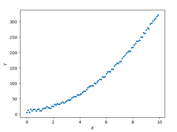
如果我们想用高次多项式拟合上面的数据应该如何实现呢?其实很简单,设假设函数为
与之相像的线性函数为
观察(1)式和(2)式,其实我们只要把(1)式中的(x)看作是(2)式中的(x_1),(1)式中的(x^2)看作是(2)式中的(x_2),就可以把拟合一个关于(x)的二次函数的任务转换为拟合一个关于(x_1)和(x_2)的线性函数的任务,这样问题就简单了,关于如何拟合一个线性函数请参考大叔学ML第二:线性回归。
现在,我们用正规方程来拟合线性函数,正规方程形如:(vec heta=(X^TX)^{-1}X^Tvec{y}),关键在于构建特征矩阵(X),显然,特征矩阵的第一列(vec x_0)全为1,第二列(vec x_1)由样本中的属性(x)构成,第三列(vec x_2)由样本中的属性(x)的平方构成。
小试牛刀
import numpy as np
import matplotlib.pyplot as plt

''' 创建样本数据如下:'''
X = np.arange(0, 10, 0.1) # 产生100个样本
noise = np.random.randint(-5, 5, (1, 100))
Y = 10 + 2 * X + 3 * X * X + noise # 100个样本对应的标记

'''下面用正规方程求解theta'''
X0 = np.ones((100, 1)) # x0赋值1
X1 = X.reshape(100, 1) # x1
X2 = X1 * X1 #x2为x1的平方

newX = np.hstack((X0, X1, X2)) # 构建一个特征矩阵
newY = Y.reshape(100, 1) # 把标记转置一下
theta = np.dot(np.dot(np.linalg.pinv(np.dot(newX.T, newX)), newX.T), newY)
print(theta)

'''绘制'''
plt.xlabel('$X$')
plt.ylabel('$Y$')
plt.scatter(X, Y, marker='.') # 原始数据
plt.plot(X, theta[0] + theta[1] * X + theta[2] * X * X, color = 'r') # 绘制我们拟合得到的函数
plt.show()
运行结果:
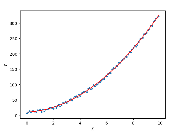
简直完美。
再试牛刀
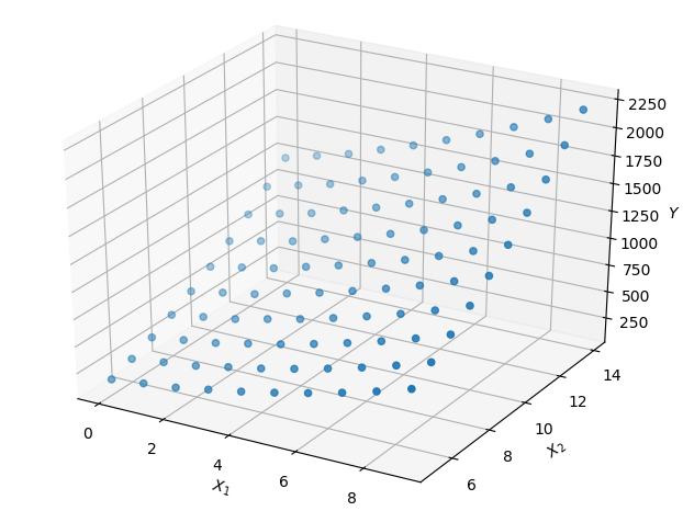
上面我们只是拟合了一个一元函数(样本数据仅包含一个元素),下面我们来尝试拟合一个二元函数。假设我们有一堆样本,每个样本有两个元素,看起来大概是这样:
我们欲拟合一个函数形式如下:
同样,对比与之相像的线性函数:
我们建立如下对应关系:
| 高次多项式 | 线性式 |
|---|---|
| (x_0=1) | (x_0=1) |
| (x_1) | (x_1) |
| (x_2) | (x_2) |
| (x_1^2) | (x_3) |
| (x_1x_2) | (x_4) |
| (x_2^2) | (x_5) |
编程如下:
import numpy as np
import matplotlib.pyplot as plt
from mpl_toolkits.mplot3d import Axes3D

# 测试用多项式
def ploy(X1, X2, *theta):
    noise = np.random.randint(-5, 5, (1, 10))
    Y = theta[0] + theta[1] * X1 + theta[2] * X2 + theta[3] * X1**2 + theta[4] * X1 * X2 + theta[5] * X2**2 + noise # 10个样本对应的标记
    return Y

''' 创建样本数据如下 '''
X1 = np.arange(0, 10, 1) # 产生10个样本的第一个属性
X2 = np.arange(5, 15, 1) # 产生10个样本的第二个属性
Y = ploy(X1, X2, 1, 2, 3, 4, 5, 6)

'''构建特征矩阵 '''
newX0 = np.ones((10, 1))
newX1 = np.reshape(X1, (10, 1))
newX2 = np.reshape(X2, (10, 1))
newX3 = np.reshape(X1**2, (10, 1))
newX4 = np.reshape(X1 * X2, (10, 1))
newX5 = np.reshape(X2**2, (10, 1))

newX = np.hstack((newX0, newX1, newX2, newX3, newX4, newX5)) # 特征矩阵

'''用正规方程拟合 '''
newY = Y.reshape(10, 1) #把标记转置一下
result = np.dot(np.dot(np.linalg.pinv(np.dot(newX.T, newX)), newX.T), newY)
theta = tuple(result.reshape((1, 6))[0].tolist())
print(theta)

'''绘制 '''
fig = plt.figure()
ax = Axes3D(fig)
ax.set_xlabel('$X_1$')
ax.set_ylabel('$X_2$')
ax.set_zlabel('$Y$')
AxesX1, AxesX2 = np.meshgrid(X1, X2)

AxesY = ploy(AxesX1, AxesX2, 1, 2, 3, 4, 5, 6) # 原始数据
ax.scatter(AxesX1, AxesX2, AxesY)

regressionY = ploy(AxesX1, AxesX2, *theta) # 用拟合出来的theta计算数据
ax.plot_surface(AxesX1, AxesX2, regressionY, color='r', alpha='0.5')
plt.show()
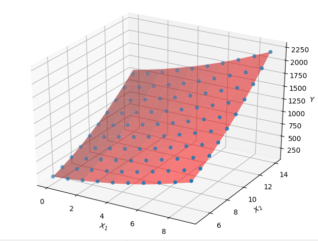
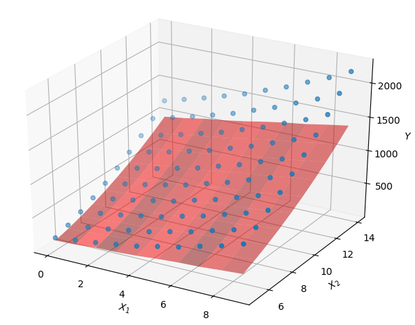
运行结果:
调用类库
我们可以调用sklean中模块PolynomialFeatures自动生成特征矩阵,而无需自己创建,计算参数(vec heta)也不用自己写,而是使用sklean中的模块linear_model:
import numpy as np
import matplotlib.pyplot as plt
from sklearn.preprocessing import PolynomialFeatures
from sklearn import linear_model
from mpl_toolkits.mplot3d import Axes3D

# 测试用多项式
def ploy(X1, X2, *theta):
    noise = np.random.randint(-5, 5, (1, 10))
    Y = theta[0] + theta[1] * X1 + theta[2] * X2 + theta[3] * X1**2 + theta[4] * X1 * X2 + theta[5] * X2**2 + noise # 10个样本对应的标记
    return Y

''' 创建样本数据如下 '''
X1 = np.arange(0, 10, 1) # 产生10个样本的第一个属性
X2 = np.arange(5, 15, 1) # 产生10个样本的第二个属性
Y = ploy(X1, X2, 1, 2, 3, 4, 5, 6)

X = np.vstack((X1, X2)).T
Y = Y.reshape((10, 1))

'''构建特征矩阵 '''
poly = PolynomialFeatures(2)
features_matrix = poly.fit_transform(X)
names = poly.get_feature_names()

''' 拟合'''
regr = linear_model.LinearRegression()
regr.fit(features_matrix, Y)

theta = tuple(regr.intercept_.tolist() + regr.coef_[0].tolist())
print(theta)

'''绘制 '''
fig = plt.figure()
ax = Axes3D(fig)
ax.set_xlabel('$X_1$')
ax.set_ylabel('$X_2$')
ax.set_zlabel('$Y$')
AxesX1, AxesX2 = np.meshgrid(X1, X2)

AxesY = ploy(AxesX1, AxesX2, 1, 2, 3, 4, 5, 6) # 原始数据
ax.scatter(AxesX1, AxesX2, AxesY)

regressionY = ploy(AxesX1, AxesX2, *theta) # 用拟合出来的theta计算数据
ax.plot_surface(AxesX1, AxesX2, regressionY, color='r', alpha='0.5')
plt.show()
运行结果如下:
感觉还不让自己写的代码拟合的好,可能是大叔的样本太少?或者是其他什么原因导致。大叔现在功力还不深,等有空了会看看这些类库的源码。
至于何时必须自己编码而不是调用类库,大叔在上文末尾做了一点总结,不一定对,欢迎指正。祝大家周末愉快。