TensorFlow学习笔记（六）循环神经网络

一、循环神经网络简介

　　循环神经网络的主要用途是处理和预测序列数据。循环神经网络刻画了一个序列当前的输出与之前信息的关系。从网络结构上，循环神经网络会记忆之前的信息，并利用之前的信息影响后面节点的输出。

下图展示了一个典型的循环神经网络。

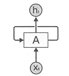
循环神经网络的一个重要的概念就是时刻。上图中循环神经网络的主体结构A的输入除了来自输入层的Xt，还有一个自身当前时刻的状态St。

在每一个时刻，A会读取t时刻的输入Xt，并且得到一个输出Ht。同时还会得到一个当前时刻的状态St，传递给下一时刻t+1。

因此，循环神经网络理论上可看作同一神经结构被无限重复的过程。（无限重复目前还是不可行的）

将循环神经网络按照时间序列展开，如下图所示

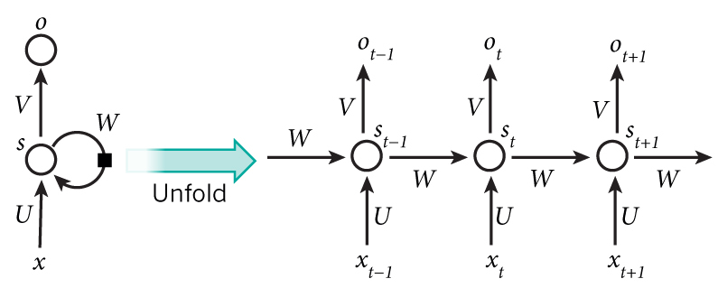
 xt是t时刻的输入

St是t时刻的“记忆”，St = f（WSt-1 + Uxt），f是tanh等激活函数

Ot 是t时刻的输出

下图给出一个最简单的循环体或者叫记忆体的结构图

 

下图展示了一个循环神经网络的前向传播算法的具体计算过程。

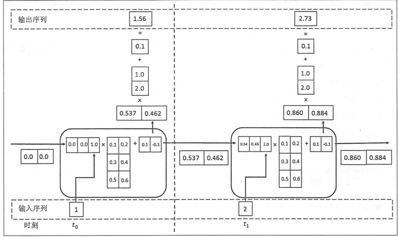
在得到前向传播计算结果之后，可以和其他网络类似的定义损失函数。神经网络的唯一区别在于它每一个时刻都有一个输出，所以循环神经网络的总损失为前面所有时刻的损失函数的总和。

我们利用代码来实现这个简单的前向传播过程。

import numpy as np

X = [1,2]
state = [0.0,0.0]
#定义不同输入部分的权重
w_cell_state = np.asarray([[0.1,0.2],[0.3,0.4]])
w_cell_input = np.asarray([0.5,0.6])
b_cell = np.asarray([0.1,-0.1])
#定义输出层的权重
w_output = np.asarray([[0.1],[0.2]])
b_output = 0.1
#按照时间顺序执行循环神经网络的前向传播过程
for i in range(len(X)):
    before_activetion = np.dot(state,w_cell_state) + X[i] * w_cell_input + b_cell
    state = np.tanh(before_activetion)
    #计算当前时刻的最终输出
    final_output = np.dot(state,w_output) + b_output
    #输出每一时刻的信息
    print("before_activation",before_activetion)
    print("state",state)
    print("final_output",final_output)

二、长短时记忆网络（LSTM）结构

循环神经网络工作的关键点就是使用历史的信息来帮助当前的决策。循环神经网络能很好的利用传统的神经网络不能建模的信息，但同时，也带来了更大的挑战——长期依赖的问题。

　　在有些问题中，模型仅仅需要短期内的信息来执行当前的任务。但同时也会有一些上下文场景更加复杂的情况。当间隔不断增大时，简单的循环神经网络可能会丧失学习到如此远的信息的能力。或者在复杂的语言场景中，有用的信息的间隔有大有小，长短不一，循环神经网络的性能也会受限。

　　为了解决这类问题，设计了LSTM。与单一tanh循环结构不同，LSTM拥有三个门：“输入门”、“输出门”、“遗忘门”。 

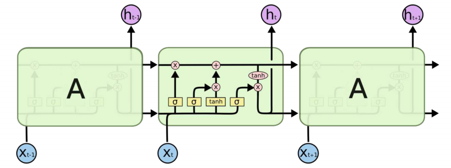
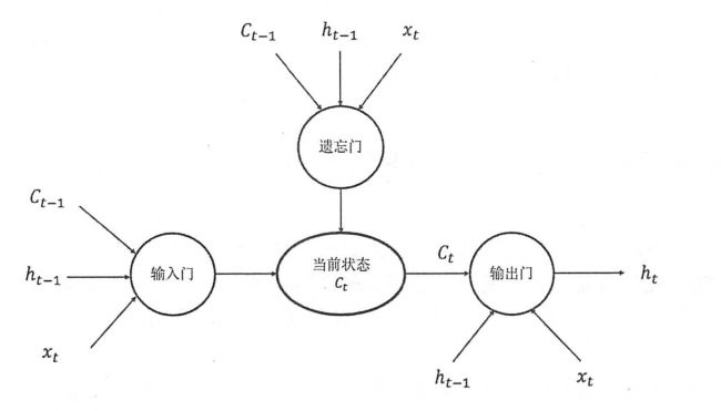
　　LSTM靠这些“门”的结构信息有选择的影响循环神经网络中每个时刻的状态。所谓的“门”就是一个sigmod网络和一个按位做乘法的操作。当sigmod输出为1时，全部信息通过；为0时，信息无法通过。为了使循环神经网络更有效的保持长期记忆。“遗忘门“和”输入门”就至关重要。“遗忘门”就是让神经网络忘记之前没有用的信息。从当前的输入补充新的“记忆”是“输入门”作用。

使用LSTM结构的循环神经网络的前向传播时一个比较复杂的计算过程。在TensorFlow中可以被很简单的实现。例如下面的伪代码：

import tensorflow as tf

#定义一个LSTM结构。TF通过一句简单的命令就可以定义一个LSTM循环体
#LSTM中使用的变量也会自动声明

lstm = tf.nn.rnn_cell.BasicLSTMCell(lstm_hidden_size)
#将LSTM中的状态初始化问哦全0数组。
#BasicLSTMCell类提供了zero_state函数来生成全0 的初始状态
state = lstm.zero_state(batch_size,tf.float32)
current_input = "hello"
#定义损失函数
loss = 0.0
#虽然rnn理论上可以处理任意长度的序列，但是在训练时为了避免梯度消散的问题，会规定一个最大的循环长度num_temps
for i in range(num_temps):
    #在第一个时刻声明LSTM结构中使用的变量，在之后的时刻都需要服用之前的定义好的变量。
    if i > 0:
        tf.get_variable_scope().reuse_variables()
    #每一步处理时间序列中的一个时刻
    lstm_output,state = lstm(current_input,state)
    #将当前时刻LSTM结构的输出传入一个全连接层得到最后的输出
    final_output = full_connected(lstm_output)
    #计算当前时刻的输出的损失
    loss += calc_loss(final_output,expected_output)

#利用BP后向传播算法训练模型

三、循环神经网络的变种

1、双向循环神经网络和深层循环神经网络

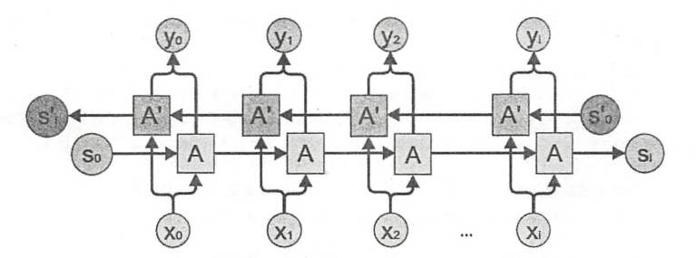
在经典的循环神经网络中，状态的传输时从前向后单向的。然而，在有些问题中，当前时刻的输出不仅和之前的状态有关，也和之后的转台有关。只是后就需要使用双向循环神经网络来解决此类问题。双向循环神经网络时由连个神经网络上下叠加在一起组成的。输出有这两个神经网络的转台共同决定的。下图展示了一个双向循环神经网络。

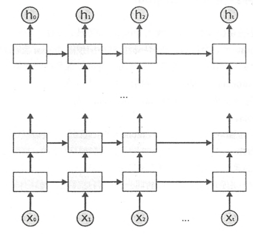
深层循环神经网络是循环神经网络的另外一种变体。为了增强模型的表达能力，可以将每一时刻上的循环体重复多次。深层循环神经网络在每一时刻上将循环体结构重复了多次。 每一层循环体中的参数是一致的，不同层的循环体参数可以不一致。TF提供了MultiRNNCell类来实现深层循环神经网络的前向传播过程。

import tensorflow as tf

#定义一个基本的LSTM结构作为循环体的基础结构，深层循环神经网络也可以支持其他的循环提结构
lstm = tf.nn.rnn_cell.BasicLSTMCell(lstm_size)

#通过MultiRNNCell类来实现深层循环神经网络中每一时刻的前向传播过程。其中。number_of_layers 表示了有多少层，也就是图
#中从xi到hi需要经过多少个LSTM结构。
stacked_lstm = tf.nn.rnn_cell.MultiRNNCell([lstm]*number_of_layers)
#和经典神经网络一样，可以通过zero_state函数获得初始状态。
state = stacked_lstm.zero_state(batch_size,tf.float32)
#计算每一时刻的前向传播过程
for i in range(num_steps):
    if i > 0:
        tf.get_variable_scope().reuse_variables()
    stacked_lstm_output  ,state = stacked_lstm(current_input,state)
    final_output =  fully_connected(stacked_lstm_output)
    loss += calc_loss(final_output,expected_output)
    

2、循环神经网络的dropout

　　dropout可以样循环神经网络更加的健壮。dropout一般只在不同层循环体之间使用。也就是说从t-1时刻传递到时刻t，RNN不会进行状态的dropout，而在同一时刻t，不同层循环体之间会使用dropout。

在TF中，使用tf.nn.rnn_cell.DropoutWrapper类可以很容易实现dropout功能。

#定义LSTM结构
lstm  = tf.nn.rnn_cell.BasicLSTMCell(lstm_size)
#通过DropoutWrapper来实现dropout功能。input_keep_drop参数用来控制输入的dropout的概率，output_keep_drop参数用来控制输出的dropout的概率，
dropout_lstm = tf.nn.rnn_cell.DropoutWrapper(lstm,input_keep_prob=0.5,output_keep_prob=0.5)
#在使用了dropout的基础上定义深层RNN
stacked_lstm = tf.nn.rnn_cell.MultiRNNCell([dropout_lstm]* 5)

四、循环神经网络的样例应用

1、自然语言建模

　　简单的说，语言模型的目的就是为了计算一个句子的出现概率。在这里把句子看成单词的序列S = （w1,w2,w3....wm），其中m为句子的长度，它的概率可以表示为

P（S） = p（w1，w2,w3.....wm） = p(w1)p(w2|w1)p(w3|w1,w2)p(wm| w1,w2...wm)

等式右边的每一项都是语言模型中的一个参数。为了估计这些参数的取值，常用的方法有n-gram、决策树、最大熵模型、条件随机场、神经网络模型。

　　语言模型效果的好坏的常用的评价指标是复杂度（perplexity）。简单来说，perplexity刻画的就是通过某一语言模型估计一句话出现的概率。值越小越好。复杂度的计算公式：

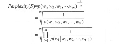
下面就利用语言模型来处理PTB数据集。

为了让PTB数据集使用更方便，TF提供了两个函数来预处理PTB数据集。ptb_raw_data用来读取原始数据，并将原始数据的单词转化为单词ID，形成一个非常长的序列。ptb_iterator将序列按照某固定的长度来截断，并将数据组成batch。

使用循环神经网络实现语言模型

# -*- coding:utf-8 -*-

import numpy as np
import tensorflow as tf
from tensorflow.models.rnn.ptb import reader
from tensorflow.contrib.legacy_seq2seq import sequence_loss_by_example
DATA_PATH = "path/to/ptb/data"
HIDDEN_SIZE = 200 #隐藏层的规模
NUM_LAYERS = 2 #DRNN中LSTM结构的层数
VOCAB_SIZE = 10000 #词典规模，加上语句结束符和稀有单词结束符总共10000
LEARNING_RATE = 1.0
TRAIN_BATCH_SIZE = 20  #训练数据BATCH大小
TRAIN_NUM_STEPS = 35    #训练数据截断长度
#在测试的时候不需要使用截断
EVAL_BATCH_SIZE = EVAL_NUM_STEP = 1
NUM_EPOCH = 2 #使用训练数据的轮数
KEEP_DROP =0.5 #节点不被dropout的概率
MAX_GRAD_NORM =5 #用于控制梯度膨胀的参数


#定义一个PTBMODEL类来描述模型，方便维护循环神经网络中的状态
class PTBMODEL:
    def __init__(self,batch_size,num_steps,is_training = True):
        self.batch_size = batch_size
        self.num_steps = num_steps
        #定义输入层，维度为batch_size* num_steps
        self.input_data = tf.placeholder(tf.int32,shape=[batch_size,num_steps])
        #定义预期输出。它的维度和ptb_iterrattor输出的正确答案维度是一样的。
        self.targets = tf.placeholder(tf.int32,[batch_size,num_steps])
        #定义使用LSTM结构为循环体结构且使用dropout的深层循环神经网络
        lstm_cell = tf.nn.rnn_cell.BasicLSTMCell(HIDDEN_SIZE)
        if is_training:
            lstm_cell = tf.nn.rnn_cell.DropoutWrapper(lstm_cell,output_keep_prob=KEEP_DROP)
        cell = tf.nn.rnn_cell.MultiRNNCell(lstm_cell)
        #初始化初始状态
        self.initial_state = cell.zero_state(batch_size,tf.float32)
        #将单词ID转换为单词向量，总共有VOCAB_SIZE个单词，每个单词向量的维度为HIDDEN_SIZE，所以embedding参数的维度为
        #VOCAB_SIZE*HIDDEN_SIZE
        embedding = tf.get_variable("embedding",[VOCAB_SIZE,HIDDEN_SIZE])
        #将原本batch_size * num_steps个单词ID转化为单词向量，转化后的输入层维度为batch_size * num_steps * HIDDEN_SIZE
        inputs = tf.nn.embedding_lookup(embedding,self.input_data)
        #只在训练时使用dropout
        if is_training:
            inputs  = tf.nn.dropout(inputs,KEEP_DROP)
        #定义输出列表，在这里现将不同时刻LSTM结构的输出收集起来，再通过一个全连接层得到最终输出
        output = []
        #state 存储不同batch中LSTM的状态，并且初始化为0.
        state = self.initial_state
        with tf.variable_scope("RNN"):
            for time_step  in range(num_steps):
                if time_step > 0 :
                    tf.get_variable_scope().reuse_variables()
                cell_output,state = cell(inputs[:,time_step,:],state)
                #将当前输出加入输出队列
                output.append(cell_output)
        #把输出队列展开成[batch,hidden_size*num_steps]的形状，然后再reshape成【batch*num_steps,hidden_size】的形状。
        output = tf.reshape(tf.concat(output,1),[-1,HIDDEN_SIZE])
        #将从LSTM中得到的输出再经过一个全连接层得到最后的预测结果，最终的预测结果在每一时刻上都是一个长度为VOCAB_SIZE的数组
        #经过SoftMax层之后表示下一个位置是不同单词的概率。
        weight = tf.get_variable("weight",[HIDDEN_SIZE,VOCAB_SIZE])
        baias  =  tf.get_variable("bias",[VOCAB_SIZE])
        logits = tf.matmul(output,weight) + baias
        #定义交叉熵损失函数
        loss  = sequence_loss_by_example([logits],[tf.reshape(self.targets,[-1])],
                                                                   [tf.ones([batch_size*num_steps],dtype=tf.float32)]
                                                                   )
        #计算得到每个batch的平均损失
        self.cost = tf.reduce_sum(loss)/batch_size
        self.final_state = state
        #只在训练模型是定义反向传播操作
        if not is_training:
            return

        trainable_variables = tf.trainable_variables()
        #通过clip_by_global_norm函数控制梯度的大小，避免梯度膨胀的问题
        grads,_ = tf.clip_by_global_norm(tf.gradients(self.cost,trainable_variables),MAX_GRAD_NORM)
        #定义优化方法
        optimizer = tf.train.GradientDescentOptimizer(LEARNING_RATE)
        #定义训练步骤
        self.train_op = optimizer.apply_gradients(zip(grads,trainable_variables))

#使用给定的模型model在数据data上运行train_op并返回全部数据上的perplexity值

def run_epoch(session,model,data,train_op,output_log):
    #计算perplexity的辅助变量
    total_costs = 0.0
    iters = 0
    state = session.run(model.initial_state)
    #使用当前数据训练或者测试模型
    for step ,(x,y) in  enumerate(reader.ptb_iterator( data,model.batch_size,model.num_steps)):
        cost,state,_ = session.run([model.cost,model.final_output,model.train_op],{
            model.input_data:x,model.targets:y,
            model.initial_state:state
        })
        total_costs += cost
        iters += model.num_steps
        #只有在训练时输出日志
        if output_log and step % 100 == 0:
            print("After %s steps ,perplexity is %.3f"%(step,np.exp(total_costs/iters)))

    #返回给定模型在给定数据上的perplexity
    return np.exp(total_costs/iters)


def main(_):
    #获取原始数据
    train_data,valid_data,test_data = reader.ptb_raw_data(DATA_PATH)
    #定义初始化函数
    initializer = tf.random_uniform_initializer(-0.05,0.05)
    #定义训练用的循环神经网络模型
    with tf.variable_scope("language_model",reuse=True,initializer=initializer):
        train_model = PTBMODEL(TRAIN_BATCH_SIZE,TRAIN_NUM_STEPS,is_training=True)
    #定义评估用的循环神经网络模型
    with tf.variable_scope("language_model",reuse=True,initializer=initializer):
        eval_model = PTBMODEL(EVAL_BATCH_SIZE,EVAL_NUM_STEP,is_training=False)
    with tf.Session() as sess:
        tf.global_variables_initializer().run()
        #使用训练数据训练模型
        for i in range(NUM_EPOCH):
            print("In iteration:%s"%(i+1))
            #在所有训练数据上训练RNN
            run_epoch(sess,train_model,train_data,train_model.train_op,True)
            #使用验证集评测模型效果
            valid_perplexity = run_epoch(sess,eval_model,valid_data,tf.no_op(),False)
            print("Epoch %s ,Validation perplexity :%.3f"%(i+1,valid_perplexity))
        # 最后使用测试集验证模型效果
        test_perplexity = run_epoch(sess,eval_model,valid_data,tf.no_op(),False)
        print("TEST perplexity :%.3f"%(test_perplexity))

if __name__ == '__main__':
    tf.app.run()

 四、时间序列预测

 　　怎么用循环神经网络来预测正弦函数，可利用TF的高级封装--TFLearn.

　　1、使用TFLearn自定义模型

　　

from sklearn  import cross_validation
from sklearn import datasets
from sklearn import metrics
import tensorflow as tf
from tensorflow.contrib.learn import models,Estimator,SKCompat
from tensorflow.contrib import layers,framework
import numpy as np
#导入TFLearn

#自定义模型，对于给定的输入数据以及其对应的正确答案，返回在这些输入上的预测值、损失值以及训练步骤
def my_model(feature,target):
    #将预测的模型转换为one-hot编码的形式，因为共有三个类别，所以向量长度为3.经过转化后，三个个类别（1，0，0），（0，1，0），（0，0，1）
    target = tf.one_hot(target,3,1,0)
    #定义模型以及其在给定数据上的损失函数。TFLearn通过logistic_regression封装了一个单层全链接神经网络
    logits,loss = models.logistic_regression(feature,target)
    #创建模型的优化器，并得到优化步骤
    train_op = layers.optimize_loss(loss,   #损失函数
                                    framework.get_global_step(), #获取训练步数并在训练时更新
                                    optimizer="Adagrad",  #定义优化器
                                    learning_rate=0.1 #定义学习率
                                    )
    #返回在给定数据上的预测结果、损失值以及优化步骤
    return tf.argmax(logits,1) ,loss,train_op

#加载iris数据集，并划分为训练集合和测试集合
iris  = datasets.load_iris()
x_train,x_test,y_train,y_test = cross_validation.train_test_split(iris.data,iris.target,test_size=0.2,random_state=0)
#对自定义的模型进行封装
classifier =Estimator(model_fn=my_model)
classifier = SKCompat(classifier)
#使用封装好的模型和训练数据执行100轮的迭代
classifier.fit(x_train,y_train,steps=100)
#使用训练好的模型进行预测
y_predicted = classifier.predict(x_test)



#计算模型的准确度
score  = metrics.accuracy_score(y_test,y_predicted)
print("Accuracy: %.2f %%"%(score * 100))

2、预测正选函数

　　因为标准的RNN预测的是离散值，所以程序需要将连续的sin函数曲线离散化。

　　每个SAMPLE_ITERVAL对sin函数进行一次采样，采样得到的序列就是sin函数离散化之后的结果

import numpy as np
import tensorflow as tf
import matplotlib as mpl
from matplotlib import pyplot as plt
from tensorflow.contrib.learn.python.learn.estimators.estimator import SKCompat

# TensorFlow的高层封装TFLearn
learn = tf.contrib.learn

# 神经网络参数
HIDDEN_SIZE = 30  # LSTM隐藏节点个数
NUM_LAYERS = 2  # LSTM层数
TIMESTEPS = 10  # 循环神经网络截断长度
BATCH_SIZE = 32  # batch大小

# 数据参数
TRAINING_STEPS = 3000  # 训练轮数
TRAINING_EXAMPLES = 10000  # 训练数据个数
TESTING_EXAMPLES = 1000  # 测试数据个数
SAMPLE_GAP = 0.01  # 采样间隔


def generate_data(seq):
    # 序列的第i项和后面的TIMESTEPS-1项合在一起作为输入，第i+TIMESTEPS项作为输出
    X = []
    y = []
    for i in range(len(seq) - TIMESTEPS - 1):
        X.append([seq[i:i + TIMESTEPS]])
        y.append([seq[i + TIMESTEPS]])
    return np.array(X, dtype=np.float32), np.array(y, dtype=np.float32)


# LSTM结构单元
def LstmCell():
    lstm_cell = tf.contrib.rnn.BasicLSTMCell(HIDDEN_SIZE)
    return lstm_cell


def lstm_model(X, y):
    # 使用多层LSTM，不能用lstm_cell*NUM_LAYERS的方法，会导致LSTM的tensor名字都一样
    cell = tf.contrib.rnn.MultiRNNCell([LstmCell() for _ in range(NUM_LAYERS)])

    # 将多层LSTM结构连接成RNN网络并计算前向传播结果
    output, _ = tf.nn.dynamic_rnn(cell, X, dtype=tf.float32)
    output = tf.reshape(output, [-1, HIDDEN_SIZE])

    # 通过无激活函数的全联接层计算线性回归，并将数据压缩成一维数组的结构
    predictions = tf.contrib.layers.fully_connected(output, 1, None)

    # 将predictions和labels调整为统一的shape
    y = tf.reshape(y, [-1])
    predictions = tf.reshape(predictions, [-1])

    # 计算损失值
    loss = tf.losses.mean_squared_error(predictions, y)

    # 创建模型优化器并得到优化步骤
    train_op = tf.contrib.layers.optimize_loss(
        loss,
        tf.train.get_global_step(),
        optimizer='Adagrad',
        learning_rate=0.1)

    return predictions, loss, train_op


# 用sin生成训练和测试数据集
test_start = TRAINING_EXAMPLES * SAMPLE_GAP
test_end = (TRAINING_EXAMPLES + TESTING_EXAMPLES) * SAMPLE_GAP
train_X, train_y = generate_data(
    np.sin(np.linspace(0, test_start, TRAINING_EXAMPLES, dtype=np.float32)))
test_X, test_y = generate_data(
    np.sin(
        np.linspace(test_start, test_end, TESTING_EXAMPLES, dtype=np.float32)))

# 建立深层循环网络模型
regressor = SKCompat(learn.Estimator(model_fn=lstm_model, model_dir='model/'))

# 调用fit函数训练模型
regressor.fit(train_X, train_y, batch_size=BATCH_SIZE, steps=TRAINING_STEPS)

# 使用训练好的模型对测试集进行预测
predicted = [[pred] for pred in regressor.predict(test_X)]

# 计算rmse作为评价指标
rmse = np.sqrt(((predicted - test_y)**2).mean(axis=0))
print('Mean Square Error is: %f' % (rmse[0]))

# 对预测曲线绘图，并存储到sin.jpg
fit = plt.figure()
plot_predicted = plt.plot(predicted,label = "predicted")
plot_test = plt.plot(test_y,label = "real_sin")
plt.legend([plot_predicted, plot_test], ['predicted', 'real_sin'])

plt.savefig("sin.png")