数据集及源码获取链接:
链接:https://pan.baidu.com/s/13UGowU3SRLn2EDwFLJBU_Q
提取码:690o
一、使用 Mnist 数据集,使用 softmax 识别数字
1.导入所需模块
from keras import models
from keras import layers
from keras.utils import to_categorical
import pandas as pd
import matplotlib.pyplot as plt
import numpy as np
Using TensorFlow backend.
2.载入数据
train = pd.read_csv('mnist/mnist_train.csv',header = None)
test = pd.read_csv('mnist/mnist_test.csv',header = None)
print(train.shape)
print(test.shape)
(60000, 785)
(10000, 785)
train_data = train.iloc[:,1:]
test_data = test.iloc[:,1:]
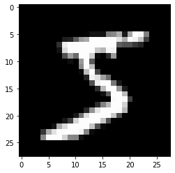
# 画出第一个训练样本的图像
train_data = np.array(train_data)
image = train_data[0].reshape(28,28)
plt.imshow(image,cmap ='gray')
plt.show()
# 画出第一个测试样本的图像
test_data = np.array(test_data)
image = test_data[0].reshape(28,28)
plt.imshow(image,cmap ='gray')
plt.show()

train_label=train.iloc[:,0]
test_label = test.iloc[:,0]
print(train_label.shape)
print(test_label.shape)
(60000,)
(10000,)
train_label[0]
5
test_label[0]
7
train_image = np.array(train_data)
test_image = np.array(test_data)
train_labels = np.array(train_label)
test_labels = np.array(test_label)
train_image.shape
(60000, 784)
test_labels
array([7, 2, 1, ..., 4, 5, 6], dtype=int64)
3.数据预处理
将像素值缩放到[0,1]之间
train_image = train_image.astype('float32')/255
test_image = test_image.astype('float32')/255
标签分类编码(one-hot)
train_labels = to_categorical(train_labels)
test_labels = to_categorical(test_labels)
train_labels
array([[0., 0., 0., ..., 0., 0., 0.],
       [1., 0., 0., ..., 0., 0., 0.],
       [0., 0., 0., ..., 0., 0., 0.],
       ...,
       [0., 0., 0., ..., 0., 0., 0.],
       [0., 0., 0., ..., 0., 0., 0.],
       [0., 0., 0., ..., 0., 1., 0.]], dtype=float32)
4.构建网络
network = models.Sequential()
network.add(layers.Dense(512,activation='relu',input_shape=(train_image.shape[-1],)))
network.add(layers.Dense(10,activation='softmax'))
network.compile(optimizer='rmsprop',loss='categorical_crossentropy',metrics=['accuracy'])
network.summary()
Model: "sequential_1"
_________________________________________________________________
Layer (type)                 Output Shape              Param #
=================================================================
dense_1 (Dense)              (None, 512)               401920
_________________________________________________________________
dense_2 (Dense)              (None, 10)                5130
=================================================================
Total params: 407,050
Trainable params: 407,050
Non-trainable params: 0
_________________________________________________________________
第一层:(784+1)*512 = 401920
第二层:(512+1)*10 = 5130
5.训练网络
留出10000个样本作为验证集
train_image.shape
(60000, 784)
x_val = train_image[:10000]
partial_x_train = train_image[10000:]

y_val = train_labels[:10000]
partial_y_train = train_labels[10000:]
x_val.shape
(10000, 784)
partial_x_train.shape
(50000, 784)
训练模型
history = network.fit(partial_x_train,
                    partial_y_train,
                    epochs=30,
                     batch_size=512,
                     validation_data = (x_val,y_val))
Train on 50000 samples, validate on 10000 samples
Epoch 1/30
50000/50000 [==============================] - 3s 53us/step - loss: 0.4245 - accuracy: 0.8808 - val_loss: 0.2334 - val_accuracy: 0.9368
Epoch 2/30
50000/50000 [==============================] - 3s 61us/step - loss: 0.1908 - accuracy: 0.9448 - val_loss: 0.1645 - val_accuracy: 0.9525
Epoch 3/30
50000/50000 [==============================] - 3s 57us/step - loss: 0.1334 - accuracy: 0.9613 - val_loss: 0.1312 - val_accuracy: 0.9629
Epoch 4/30
50000/50000 [==============================] - 2s 43us/step - loss: 0.0988 - accuracy: 0.9712 - val_loss: 0.1136 - val_accuracy: 0.9680
Epoch 5/30
50000/50000 [==============================] - 3s 51us/step - loss: 0.0781 - accuracy: 0.9774 - val_loss: 0.0956 - val_accuracy: 0.9726
Epoch 6/30
50000/50000 [==============================] - 3s 57us/step - loss: 0.0613 - accuracy: 0.9819 - val_loss: 0.1033 - val_accuracy: 0.9691
Epoch 7/30
50000/50000 [==============================] - 2s 43us/step - loss: 0.0506 - accuracy: 0.9854 - val_loss: 0.0799 - val_accuracy: 0.9770
Epoch 8/30
50000/50000 [==============================] - 2s 42us/step - loss: 0.0416 - accuracy: 0.9877 - val_loss: 0.0822 - val_accuracy: 0.9744
Epoch 9/30
50000/50000 [==============================] - 3s 50us/step - loss: 0.0338 - accuracy: 0.9909 - val_loss: 0.0726 - val_accuracy: 0.9780
Epoch 10/30
50000/50000 [==============================] - 3s 67us/step - loss: 0.0274 - accuracy: 0.9928 - val_loss: 0.0733 - val_accuracy: 0.9785
Epoch 11/30
50000/50000 [==============================] - 2s 44us/step - loss: 0.0225 - accuracy: 0.9945 - val_loss: 0.0800 - val_accuracy: 0.9771
Epoch 12/30
50000/50000 [==============================] - 2s 44us/step - loss: 0.0189 - accuracy: 0.9951 - val_loss: 0.0715 - val_accuracy: 0.9787
Epoch 13/30
50000/50000 [==============================] - 2s 44us/step - loss: 0.0154 - accuracy: 0.9963 - val_loss: 0.0731 - val_accuracy: 0.9796
Epoch 14/30
50000/50000 [==============================] - 2s 45us/step - loss: 0.0125 - accuracy: 0.9974 - val_loss: 0.0761 - val_accuracy: 0.9797
Epoch 15/30
50000/50000 [==============================] - 2s 45us/step - loss: 0.0106 - accuracy: 0.9977 - val_loss: 0.0769 - val_accuracy: 0.9778
Epoch 16/30
50000/50000 [==============================] - 2s 46us/step - loss: 0.0083 - accuracy: 0.9983 - val_loss: 0.0717 - val_accuracy: 0.9802
Epoch 17/30
50000/50000 [==============================] - 2s 46us/step - loss: 0.0069 - accuracy: 0.9987 - val_loss: 0.0730 - val_accuracy: 0.9810
Epoch 18/30
50000/50000 [==============================] - 2s 46us/step - loss: 0.0053 - accuracy: 0.9991 - val_loss: 0.0860 - val_accuracy: 0.9785
Epoch 19/30
50000/50000 [==============================] - 2s 46us/step - loss: 0.0045 - accuracy: 0.9993 - val_loss: 0.0958 - val_accuracy: 0.9752
Epoch 20/30
50000/50000 [==============================] - 2s 45us/step - loss: 0.0042 - accuracy: 0.9992 - val_loss: 0.0801 - val_accuracy: 0.9799
Epoch 21/30
50000/50000 [==============================] - 2s 46us/step - loss: 0.0032 - accuracy: 0.9995 - val_loss: 0.0782 - val_accuracy: 0.9818
Epoch 22/30
50000/50000 [==============================] - 2s 46us/step - loss: 0.0024 - accuracy: 0.9997 - val_loss: 0.0799 - val_accuracy: 0.9804
Epoch 23/30
50000/50000 [==============================] - 2s 46us/step - loss: 0.0024 - accuracy: 0.9995 - val_loss: 0.0828 - val_accuracy: 0.9801
Epoch 24/30
50000/50000 [==============================] - 2s 46us/step - loss: 0.0017 - accuracy: 0.9997 - val_loss: 0.1002 - val_accuracy: 0.9772
Epoch 25/30
50000/50000 [==============================] - 2s 47us/step - loss: 0.0017 - accuracy: 0.9998 - val_loss: 0.0870 - val_accuracy: 0.9807
Epoch 26/30
50000/50000 [==============================] - 2s 47us/step - loss: 0.0013 - accuracy: 0.9998 - val_loss: 0.0859 - val_accuracy: 0.9816
Epoch 27/30
50000/50000 [==============================] - 2s 46us/step - loss: 0.0011 - accuracy: 0.9999 - val_loss: 0.0885 - val_accuracy: 0.9812
Epoch 28/30
50000/50000 [==============================] - 2s 49us/step - loss: 8.8928e-04 - accuracy: 0.9999 - val_loss: 0.0932 - val_accuracy: 0.9807
Epoch 29/30
50000/50000 [==============================] - 2s 45us/step - loss: 6.9267e-04 - accuracy: 0.9999 - val_loss: 0.0947 - val_accuracy: 0.9807
Epoch 30/30
50000/50000 [==============================] - 2s 46us/step - loss: 6.7444e-04 - accuracy: 0.9999 - val_loss: 0.0936 - val_accuracy: 0.9812
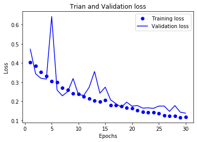
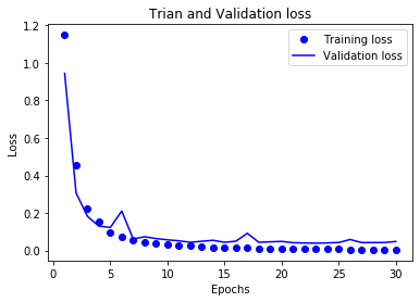
绘制损失曲线和精度曲线
history_dict = history.history
history_dict.keys()
dict_keys(['val_loss', 'val_accuracy', 'loss', 'accuracy'])
# 损失曲线
loss_values = history_dict['loss']
val_loss_values = history_dict['val_loss']
epochs = range(1,len(loss_values)+1)
plt.plot(epochs,loss_values,'bo',label='Training loss')
plt.plot(epochs,val_loss_values,'b',label='Validation loss')
plt.title('Trian and Validation loss')
plt.xlabel('Epochs')
plt.ylabel('Loss')
plt.legend()
plt.show()

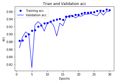
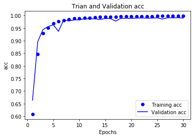
# 精度曲线
acc = history_dict['accuracy']
val_acc = history_dict['val_accuracy']
plt.plot(epochs,acc,'bo',label='Training acc')
plt.plot(epochs,val_acc,'b',label='Validation acc')
plt.title('Trian and Validation acc')
plt.xlabel('Epochs')
plt.ylabel('acc')
plt.legend()
plt.show()
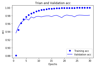
观察曲线可以发现:模型大约在训练14轮后开始过拟合
6.构建最终的网络模型
network = models.Sequential()
network.add(layers.Dense(512,activation='relu',input_shape=(train_image.shape[-1],)))
network.add(layers.Dense(10,activation='softmax'))

network.compile(optimizer='rmsprop',
                loss='categorical_crossentropy',
                metrics=['accuracy'])
history = network.fit(partial_x_train,
                    partial_y_train,
                    epochs=14,
                     batch_size=512,
                     validation_data = (x_val,y_val))
Train on 50000 samples, validate on 10000 samples
Epoch 1/14
50000/50000 [==============================] - 2s 42us/step - loss: 0.4367 - accuracy: 0.8768 - val_loss: 0.2491 - val_accuracy: 0.9299
Epoch 2/14
50000/50000 [==============================] - 2s 39us/step - loss: 0.1937 - accuracy: 0.9442 - val_loss: 0.1772 - val_accuracy: 0.9477
Epoch 3/14
50000/50000 [==============================] - 2s 39us/step - loss: 0.1323 - accuracy: 0.9623 - val_loss: 0.1525 - val_accuracy: 0.9545
Epoch 4/14
50000/50000 [==============================] - 2s 39us/step - loss: 0.0994 - accuracy: 0.9712 - val_loss: 0.1069 - val_accuracy: 0.9685
Epoch 5/14
50000/50000 [==============================] - 2s 40us/step - loss: 0.0777 - accuracy: 0.9778 - val_loss: 0.0965 - val_accuracy: 0.9706
Epoch 6/14
50000/50000 [==============================] - 2s 40us/step - loss: 0.0620 - accuracy: 0.9822 - val_loss: 0.0872 - val_accuracy: 0.9738
Epoch 7/14
50000/50000 [==============================] - 2s 39us/step - loss: 0.0501 - accuracy: 0.9855 - val_loss: 0.0797 - val_accuracy: 0.9750
Epoch 8/14
50000/50000 [==============================] - 2s 39us/step - loss: 0.0411 - accuracy: 0.9881 - val_loss: 0.0932 - val_accuracy: 0.9696
Epoch 9/14
50000/50000 [==============================] - 2s 40us/step - loss: 0.0337 - accuracy: 0.9907 - val_loss: 0.0740 - val_accuracy: 0.9765
Epoch 10/14
50000/50000 [==============================] - 2s 39us/step - loss: 0.0277 - accuracy: 0.9928 - val_loss: 0.0743 - val_accuracy: 0.9774
Epoch 11/14
50000/50000 [==============================] - 2s 39us/step - loss: 0.0231 - accuracy: 0.9938 - val_loss: 0.0740 - val_accuracy: 0.9773
Epoch 12/14
50000/50000 [==============================] - 2s 39us/step - loss: 0.0192 - accuracy: 0.9954 - val_loss: 0.0674 - val_accuracy: 0.9791
Epoch 13/14
50000/50000 [==============================] - 2s 39us/step - loss: 0.0156 - accuracy: 0.9964 - val_loss: 0.0777 - val_accuracy: 0.9788
Epoch 14/14
50000/50000 [==============================] - 2s 39us/step - loss: 0.0122 - accuracy: 0.9975 - val_loss: 0.0711 - val_accuracy: 0.9791
test_loss,test_acc = network.evaluate(test_image,test_labels)
10000/10000 [==============================] - 0s 43us/step
test_acc
0.9799000024795532
最终得到了0.98的很高的一个准确率
7.保存模型
# 保存
network.save('Dense_mnist_softmax.h5')
# 加载
# from keras.models import load_model
# load_model = load_model('cnn_mnist_softmax.h5')
8.导入自己的图片预测
导入测试图片
import cv2
test_image = cv2.imread('test.jpg',0)
plt.imshow(test_image,cmap='gray')
plt.show()
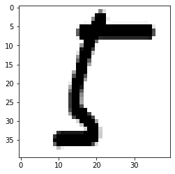
test_image.shape
(40, 40)
更改图片的尺寸为28*28
test_image = cv2.resize(test_image, (28, 28))
test_image.shape
(28, 28)
plt.imshow(test_image,cmap='gray')
plt.show()
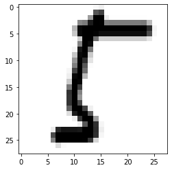
test_image = test_image.reshape(1,28*28)
颜色变换为与训练相同,背景为黑色
for i,j in enumerate(test_image[0]):
    test_image[0][i] = 255-j
plt.imshow(test_image.reshape(28,28),cmap='gray')
plt.show()

test_image.shape
(1, 784)
test_image = np.array(test_image)
test_image = test_image.astype('float32')/255
载入保存好的模型,预测测试图片
from keras.models import load_model
load_model = load_model('Dense_mnist_softmax.h5')
load_model.predict(test_image)
array([[4.90013496e-09, 3.97439243e-13, 2.33190420e-07, 7.04726277e-09,
        2.08400201e-16, 9.99991894e-01, 7.59551313e-06, 1.13947074e-10,
        2.19785747e-07, 8.43799206e-13]], dtype=float32)
result = load_model.predict_classes(test_image)[0]
print('识别出的数字为:',result)
识别出的数字为: 5
8.总结
- 选用两层卷积神经网络,
- 神经元个数为512和10,
- 激活函数为'relu'和'sigmoid',
- 训练14轮,
- 能够得到较高的准确率98%,
导入自己下载的图片,能够准确的预测出数字的内容
二、Mnist 数据集,使用 RNN 识别数字
1.导入所需模块
from keras import models
from keras import layers
from keras.utils import to_categorical
import pandas as pd
import matplotlib.pyplot as plt
import numpy as np
Using TensorFlow backend.
2.载入数据
train = pd.read_csv('mnist/mnist_train.csv',header = None)
test = pd.read_csv('mnist/mnist_test.csv',header = None)
train_data = train.iloc[:,1:]
test_data = test.iloc[:,1:]
train_label=train.iloc[:,0]
test_label = test.iloc[:,0]
train_image = np.array(train_data)
test_image = np.array(test_data)
train_labels = np.array(train_label)
test_labels = np.array(test_label)
3.数据预处理
train_image = train_image.astype('float32')/255
test_image = test_image.astype('float32')/255
train_labels = to_categorical(train_labels)
test_labels = to_categorical(test_labels)
4.构建网络与训练调优
train_image = np.array(train_image).reshape((-1, 28, 28))
test_image = np.array(test_image).reshape((-1, 28, 28))
x_val = train_image[:10000]
partial_x_train = train_image[10000:]

y_val = train_labels[:10000]
partial_y_train = train_labels[10000:]
SimpleRNN
from keras.layers import SimpleRNN

model = models.Sequential()
model.add(SimpleRNN(512,input_shape=(28, 28)))
model.add(layers.Dense(10,activation='softmax'))

model.compile(optimizer='rmsprop',
              loss='categorical_crossentropy',
              metrics=['accuracy'])
model.summary()
Model: "sequential_6"
_________________________________________________________________
Layer (type)                 Output Shape              Param #
=================================================================
simple_rnn_6 (SimpleRNN)     (None, 512)               276992
_________________________________________________________________
dense_5 (Dense)              (None, 10)                5130
=================================================================
Total params: 282,122
Trainable params: 282,122
Non-trainable params: 0
_________________________________________________________________
history = model.fit(partial_x_train,
                    partial_y_train,
                    epochs=30,
                     batch_size=512,
                     validation_data = (x_val,y_val))
Train on 50000 samples, validate on 10000 samples
Epoch 1/30
50000/50000 [==============================] - 33s 670us/step - loss: 0.4023 - accuracy: 0.8825 - val_loss: 0.4720 - val_accuracy: 0.8634
Epoch 2/30
50000/50000 [==============================] - 33s 659us/step - loss: 0.3842 - accuracy: 0.8829 - val_loss: 0.3436 - val_accuracy: 0.8923
Epoch 3/30
50000/50000 [==============================] - 31s 624us/step - loss: 0.3530 - accuracy: 0.8942 - val_loss: 0.3199 - val_accuracy: 0.9058
Epoch 4/30
50000/50000 [==============================] - 34s 684us/step - loss: 0.3321 - accuracy: 0.8998 - val_loss: 0.3159 - val_accuracy: 0.8998
Epoch 5/30
50000/50000 [==============================] - 33s 657us/step - loss: 0.3055 - accuracy: 0.9091 - val_loss: 0.6423 - val_accuracy: 0.8105
Epoch 6/30
50000/50000 [==============================] - 33s 651us/step - loss: 0.2997 - accuracy: 0.9104 - val_loss: 0.2590 - val_accuracy: 0.9241
Epoch 7/30
50000/50000 [==============================] - 36s 720us/step - loss: 0.2711 - accuracy: 0.9198 - val_loss: 0.2286 - val_accuracy: 0.9331
Epoch 8/30
50000/50000 [==============================] - 31s 622us/step - loss: 0.2601 - accuracy: 0.9234 - val_loss: 0.2513 - val_accuracy: 0.9258
Epoch 9/30
50000/50000 [==============================] - 31s 617us/step - loss: 0.2422 - accuracy: 0.9286 - val_loss: 0.3187 - val_accuracy: 0.9078
Epoch 10/30
50000/50000 [==============================] - 32s 631us/step - loss: 0.2382 - accuracy: 0.9297 - val_loss: 0.2342 - val_accuracy: 0.9301
Epoch 11/30
50000/50000 [==============================] - 31s 629us/step - loss: 0.2239 - accuracy: 0.9335 - val_loss: 0.2312 - val_accuracy: 0.9328
Epoch 12/30
50000/50000 [==============================] - 31s 617us/step - loss: 0.2141 - accuracy: 0.9362 - val_loss: 0.2736 - val_accuracy: 0.9231
Epoch 13/30
50000/50000 [==============================] - 34s 675us/step - loss: 0.2029 - accuracy: 0.9392 - val_loss: 0.3555 - val_accuracy: 0.8949
Epoch 14/30
50000/50000 [==============================] - 30s 608us/step - loss: 0.1991 - accuracy: 0.9406 - val_loss: 0.2423 - val_accuracy: 0.9291
Epoch 15/30
50000/50000 [==============================] - 30s 609us/step - loss: 0.2074 - accuracy: 0.9381 - val_loss: 0.2739 - val_accuracy: 0.9221
Epoch 16/30
50000/50000 [==============================] - 31s 614us/step - loss: 0.1805 - accuracy: 0.9464 - val_loss: 0.2076 - val_accuracy: 0.9428
Epoch 17/30
50000/50000 [==============================] - 31s 613us/step - loss: 0.1790 - accuracy: 0.9466 - val_loss: 0.1876 - val_accuracy: 0.9496
Epoch 18/30
50000/50000 [==============================] - 31s 615us/step - loss: 0.1743 - accuracy: 0.9485 - val_loss: 0.1695 - val_accuracy: 0.9502
Epoch 19/30
50000/50000 [==============================] - 31s 613us/step - loss: 0.1653 - accuracy: 0.9514 - val_loss: 0.1958 - val_accuracy: 0.9428
Epoch 20/30
50000/50000 [==============================] - 31s 615us/step - loss: 0.1630 - accuracy: 0.9517 - val_loss: 0.1748 - val_accuracy: 0.9480
Epoch 21/30
50000/50000 [==============================] - 31s 614us/step - loss: 0.1531 - accuracy: 0.9544 - val_loss: 0.1781 - val_accuracy: 0.9477
Epoch 22/30
50000/50000 [==============================] - 31s 616us/step - loss: 0.1449 - accuracy: 0.9568 - val_loss: 0.1646 - val_accuracy: 0.9524
Epoch 23/30
50000/50000 [==============================] - 31s 616us/step - loss: 0.1431 - accuracy: 0.9571 - val_loss: 0.1660 - val_accuracy: 0.9530
Epoch 24/30
50000/50000 [==============================] - 31s 615us/step - loss: 0.1413 - accuracy: 0.9580 - val_loss: 0.1634 - val_accuracy: 0.9543
Epoch 25/30
50000/50000 [==============================] - 31s 615us/step - loss: 0.1358 - accuracy: 0.9587 - val_loss: 0.1753 - val_accuracy: 0.9511
Epoch 26/30
50000/50000 [==============================] - 31s 617us/step - loss: 0.1278 - accuracy: 0.9617 - val_loss: 0.1755 - val_accuracy: 0.9486
Epoch 27/30
50000/50000 [==============================] - 30s 608us/step - loss: 0.1245 - accuracy: 0.9623 - val_loss: 0.1476 - val_accuracy: 0.9587
Epoch 28/30
50000/50000 [==============================] - 32s 642us/step - loss: 0.1228 - accuracy: 0.9617 - val_loss: 0.1779 - val_accuracy: 0.9502
Epoch 29/30
50000/50000 [==============================] - 33s 659us/step - loss: 0.1160 - accuracy: 0.9653 - val_loss: 0.1437 - val_accuracy: 0.9598
Epoch 30/30
50000/50000 [==============================] - 31s 612us/step - loss: 0.1174 - accuracy: 0.9641 - val_loss: 0.1381 - val_accuracy: 0.9604
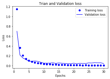
history_dict = history.history
# 损失曲线
loss_values = history_dict['loss']
val_loss_values = history_dict['val_loss']
epochs = range(1,len(loss_values)+1)
plt.plot(epochs,loss_values,'bo',label='Training loss')
plt.plot(epochs,val_loss_values,'b',label='Validation loss')
plt.title('Trian and Validation loss')
plt.xlabel('Epochs')
plt.ylabel('Loss')
plt.legend()
plt.show()
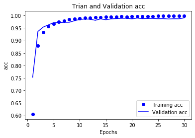
# 精度曲线
acc = history_dict['accuracy']
val_acc = history_dict['val_accuracy']
plt.plot(epochs,acc,'bo',label='Training acc')
plt.plot(epochs,val_acc,'b',label='Validation acc')
plt.title('Trian and Validation acc')
plt.xlabel('Epochs')
plt.ylabel('acc')
plt.legend()
plt.show()
test_loss,test_acc = model.evaluate(test_image,test_labels)
10000/10000 [==============================] - 6s 647us/step
test_acc
0.961899995803833
model1.save('rnn_SimpleRNN_mnist.h5')
总结:
SimpleRNN预测的准确率相比其他RNN模型更低,但也还不错
准确率为96.1%
LSTM
from keras.layers import LSTM

model1 = models.Sequential()
model1.add(LSTM(512,input_shape=(28, 28)))
model1.add(layers.Dense(10,activation='softmax'))

model1.compile(optimizer='rmsprop',
              loss='categorical_crossentropy',
              metrics=['accuracy'])
model1.summary()
Model: "sequential_7"
_________________________________________________________________
Layer (type)                 Output Shape              Param #
=================================================================
lstm_1 (LSTM)                (None, 512)               1107968
_________________________________________________________________
dense_6 (Dense)              (None, 10)                5130
=================================================================
Total params: 1,113,098
Trainable params: 1,113,098
Non-trainable params: 0
_________________________________________________________________
history = model1.fit(partial_x_train,
                    partial_y_train,
                    epochs=30,
                     batch_size=512,
                     validation_data = (x_val,y_val))
Train on 50000 samples, validate on 10000 samples
Epoch 1/30
50000/50000 [==============================] - 144s 3ms/step - loss: 1.1468 - accuracy: 0.6054 - val_loss: 0.6986 - val_accuracy: 0.7531
Epoch 2/30
50000/50000 [==============================] - 137s 3ms/step - loss: 0.3664 - accuracy: 0.8789 - val_loss: 0.2162 - val_accuracy: 0.9362
Epoch 3/30
50000/50000 [==============================] - 138s 3ms/step - loss: 0.2053 - accuracy: 0.9339 - val_loss: 0.1555 - val_accuracy: 0.9536
Epoch 4/30
50000/50000 [==============================] - 139s 3ms/step - loss: 0.1397 - accuracy: 0.9577 - val_loss: 0.1256 - val_accuracy: 0.9625
Epoch 5/30
50000/50000 [==============================] - 141s 3ms/step - loss: 0.1026 - accuracy: 0.9672 - val_loss: 0.0888 - val_accuracy: 0.9715
Epoch 6/30
50000/50000 [==============================] - 138s 3ms/step - loss: 0.0802 - accuracy: 0.9749 - val_loss: 0.0900 - val_accuracy: 0.9713
Epoch 7/30
50000/50000 [==============================] - 138s 3ms/step - loss: 0.0628 - accuracy: 0.9796 - val_loss: 0.0951 - val_accuracy: 0.9730
Epoch 8/30
50000/50000 [==============================] - 138s 3ms/step - loss: 0.0518 - accuracy: 0.9840 - val_loss: 0.0872 - val_accuracy: 0.9731
Epoch 9/30
50000/50000 [==============================] - 140s 3ms/step - loss: 0.0449 - accuracy: 0.9861 - val_loss: 0.0691 - val_accuracy: 0.9792
Epoch 10/30
50000/50000 [==============================] - 138s 3ms/step - loss: 0.0372 - accuracy: 0.9880 - val_loss: 0.0511 - val_accuracy: 0.9843
Epoch 11/30
50000/50000 [==============================] - 138s 3ms/step - loss: 0.0311 - accuracy: 0.9902 - val_loss: 0.0502 - val_accuracy: 0.9860
Epoch 12/30
50000/50000 [==============================] - 139s 3ms/step - loss: 0.0286 - accuracy: 0.9914 - val_loss: 0.0508 - val_accuracy: 0.9855
Epoch 13/30
50000/50000 [==============================] - 139s 3ms/step - loss: 0.0239 - accuracy: 0.9921 - val_loss: 0.0587 - val_accuracy: 0.9809
Epoch 14/30
50000/50000 [==============================] - 139s 3ms/step - loss: 0.0226 - accuracy: 0.9931 - val_loss: 0.0457 - val_accuracy: 0.9866
Epoch 15/30
50000/50000 [==============================] - 138s 3ms/step - loss: 0.0189 - accuracy: 0.9938 - val_loss: 0.0553 - val_accuracy: 0.9834
Epoch 16/30
50000/50000 [==============================] - 137s 3ms/step - loss: 0.0163 - accuracy: 0.9950 - val_loss: 0.0491 - val_accuracy: 0.9864
Epoch 17/30
50000/50000 [==============================] - 136s 3ms/step - loss: 0.0164 - accuracy: 0.9948 - val_loss: 0.0449 - val_accuracy: 0.9879
Epoch 18/30
50000/50000 [==============================] - 136s 3ms/step - loss: 0.0132 - accuracy: 0.9961 - val_loss: 0.0409 - val_accuracy: 0.9889
Epoch 19/30
50000/50000 [==============================] - 139s 3ms/step - loss: 0.0139 - accuracy: 0.9956 - val_loss: 0.0390 - val_accuracy: 0.9892
Epoch 20/30
50000/50000 [==============================] - 136s 3ms/step - loss: 0.0111 - accuracy: 0.9963 - val_loss: 0.0501 - val_accuracy: 0.9868
Epoch 21/30
50000/50000 [==============================] - 136s 3ms/step - loss: 0.0109 - accuracy: 0.9967 - val_loss: 0.0376 - val_accuracy: 0.9899
Epoch 22/30
50000/50000 [==============================] - 138s 3ms/step - loss: 0.0116 - accuracy: 0.9966 - val_loss: 0.0479 - val_accuracy: 0.9877
Epoch 23/30
50000/50000 [==============================] - 137s 3ms/step - loss: 0.0088 - accuracy: 0.9972 - val_loss: 0.0447 - val_accuracy: 0.9883
Epoch 24/30
50000/50000 [==============================] - 137s 3ms/step - loss: 0.0097 - accuracy: 0.9971 - val_loss: 0.0443 - val_accuracy: 0.9887
Epoch 25/30
50000/50000 [==============================] - 137s 3ms/step - loss: 0.0083 - accuracy: 0.9977 - val_loss: 0.0563 - val_accuracy: 0.9873
Epoch 26/30
50000/50000 [==============================] - 137s 3ms/step - loss: 0.0071 - accuracy: 0.9978 - val_loss: 0.0536 - val_accuracy: 0.9878
Epoch 27/30
50000/50000 [==============================] - 136s 3ms/step - loss: 0.0075 - accuracy: 0.9979 - val_loss: 0.0610 - val_accuracy: 0.9862
Epoch 28/30
50000/50000 [==============================] - 136s 3ms/step - loss: 0.0071 - accuracy: 0.9977 - val_loss: 0.0569 - val_accuracy: 0.9871
Epoch 29/30
50000/50000 [==============================] - 137s 3ms/step - loss: 0.0065 - accuracy: 0.9982 - val_loss: 0.0588 - val_accuracy: 0.9869
Epoch 30/30
50000/50000 [==============================] - 137s 3ms/step - loss: 0.0079 - accuracy: 0.9977 - val_loss: 0.0429 - val_accuracy: 0.9907
history_dict = history.history
# 损失曲线
loss_values = history_dict['loss']
val_loss_values = history_dict['val_loss']
epochs = range(1,len(loss_values)+1)
plt.plot(epochs,loss_values,'bo',label='Training loss')
plt.plot(epochs,val_loss_values,'b',label='Validation loss')
plt.title('Trian and Validation loss')
plt.xlabel('Epochs')
plt.ylabel('Loss')
plt.legend()
plt.show()
# 精度曲线
acc = history_dict['accuracy']
val_acc = history_dict['val_accuracy']
plt.plot(epochs,acc,'bo',label='Training acc')
plt.plot(epochs,val_acc,'b',label='Validation acc')
plt.title('Trian and Validation acc')
plt.xlabel('Epochs')
plt.ylabel('acc')
plt.legend()
plt.show()
test_loss,test_acc = model1.evaluate(test_image,test_labels)
10000/10000 [==============================] - 23s 2ms/step
test_acc
0.989799976348877
model1.save('rnn_LSTM_mnist.h5')
# 加载
# from keras.models import load_model
# load_model = load_model('rnn_lstm_mnist.h5')
总结:
LSTM预测的准确率很高,并且没有过拟合,但是训练时间太长了,我训练30次用了一个多小时
准确率达到了99%
GRU
from keras.layers import GRU

model2 = models.Sequential()
model2.add(GRU(512,input_shape=(28, 28)))
model2.add(layers.Dense(10,activation='softmax'))

model2.compile(optimizer='rmsprop',
              loss='categorical_crossentropy',
              metrics=['accuracy'])
model2.summary()
Model: "sequential_8"
_________________________________________________________________
Layer (type)                 Output Shape              Param #
=================================================================
gru_1 (GRU)                  (None, 512)               830976
_________________________________________________________________
dense_7 (Dense)              (None, 10)                5130
=================================================================
Total params: 836,106
Trainable params: 836,106
Non-trainable params: 0
_________________________________________________________________
history = model2.fit(partial_x_train,
                    partial_y_train,
                    epochs=30,
                     batch_size=512,
                     validation_data = (x_val,y_val))
Train on 50000 samples, validate on 10000 samples
Epoch 1/30
50000/50000 [==============================] - 131s 3ms/step - loss: 1.1481 - accuracy: 0.6081 - val_loss: 0.9439 - val_accuracy: 0.6636
Epoch 2/30
50000/50000 [==============================] - 130s 3ms/step - loss: 0.4574 - accuracy: 0.8477 - val_loss: 0.3069 - val_accuracy: 0.8961
Epoch 3/30
50000/50000 [==============================] - 130s 3ms/step - loss: 0.2251 - accuracy: 0.9302 - val_loss: 0.1818 - val_accuracy: 0.9442
Epoch 4/30
50000/50000 [==============================] - 130s 3ms/step - loss: 0.1517 - accuracy: 0.9526 - val_loss: 0.1299 - val_accuracy: 0.9563
Epoch 5/30
50000/50000 [==============================] - 130s 3ms/step - loss: 0.0980 - accuracy: 0.9695 - val_loss: 0.1230 - val_accuracy: 0.9636
Epoch 6/30
50000/50000 [==============================] - 138s 3ms/step - loss: 0.0735 - accuracy: 0.9763 - val_loss: 0.2106 - val_accuracy: 0.9374
Epoch 7/30
50000/50000 [==============================] - 133s 3ms/step - loss: 0.0562 - accuracy: 0.9819 - val_loss: 0.0615 - val_accuracy: 0.9831
Epoch 8/30
50000/50000 [==============================] - 146s 3ms/step - loss: 0.0469 - accuracy: 0.9848 - val_loss: 0.0732 - val_accuracy: 0.9787
Epoch 9/30
50000/50000 [==============================] - 138s 3ms/step - loss: 0.0365 - accuracy: 0.9888 - val_loss: 0.0638 - val_accuracy: 0.9830
Epoch 10/30
50000/50000 [==============================] - 138s 3ms/step - loss: 0.0313 - accuracy: 0.9901 - val_loss: 0.0569 - val_accuracy: 0.9831
Epoch 11/30
50000/50000 [==============================] - 141s 3ms/step - loss: 0.0267 - accuracy: 0.9916 - val_loss: 0.0518 - val_accuracy: 0.9873
Epoch 12/30
50000/50000 [==============================] - 172s 3ms/step - loss: 0.0239 - accuracy: 0.9920 - val_loss: 0.0439 - val_accuracy: 0.9871
Epoch 13/30
50000/50000 [==============================] - 187s 4ms/step - loss: 0.0209 - accuracy: 0.9936 - val_loss: 0.0493 - val_accuracy: 0.9873
Epoch 14/30
50000/50000 [==============================] - 151s 3ms/step - loss: 0.0179 - accuracy: 0.9944 - val_loss: 0.0545 - val_accuracy: 0.9849
Epoch 15/30
50000/50000 [==============================] - 133s 3ms/step - loss: 0.0145 - accuracy: 0.9956 - val_loss: 0.0438 - val_accuracy: 0.9883
Epoch 16/30
50000/50000 [==============================] - 133s 3ms/step - loss: 0.0137 - accuracy: 0.9955 - val_loss: 0.0498 - val_accuracy: 0.9882
Epoch 17/30
50000/50000 [==============================] - 132s 3ms/step - loss: 0.0138 - accuracy: 0.9959 - val_loss: 0.0919 - val_accuracy: 0.9784
Epoch 18/30
50000/50000 [==============================] - 132s 3ms/step - loss: 0.0107 - accuracy: 0.9967 - val_loss: 0.0439 - val_accuracy: 0.9892
Epoch 19/30
50000/50000 [==============================] - 131s 3ms/step - loss: 0.0115 - accuracy: 0.9967 - val_loss: 0.0464 - val_accuracy: 0.9898
Epoch 20/30
50000/50000 [==============================] - 131s 3ms/step - loss: 0.0095 - accuracy: 0.9969 - val_loss: 0.0486 - val_accuracy: 0.9893
Epoch 21/30
50000/50000 [==============================] - 131s 3ms/step - loss: 0.0089 - accuracy: 0.9972 - val_loss: 0.0416 - val_accuracy: 0.9902
Epoch 22/30
50000/50000 [==============================] - 132s 3ms/step - loss: 0.0083 - accuracy: 0.9971 - val_loss: 0.0401 - val_accuracy: 0.9906
Epoch 23/30
50000/50000 [==============================] - 132s 3ms/step - loss: 0.0084 - accuracy: 0.9975 - val_loss: 0.0390 - val_accuracy: 0.9899
Epoch 24/30
50000/50000 [==============================] - 131s 3ms/step - loss: 0.0065 - accuracy: 0.9980 - val_loss: 0.0405 - val_accuracy: 0.9902
Epoch 25/30
50000/50000 [==============================] - 131s 3ms/step - loss: 0.0066 - accuracy: 0.9980 - val_loss: 0.0426 - val_accuracy: 0.9914
Epoch 26/30
50000/50000 [==============================] - 131s 3ms/step - loss: 0.0060 - accuracy: 0.9984 - val_loss: 0.0588 - val_accuracy: 0.9863
Epoch 27/30
50000/50000 [==============================] - 131s 3ms/step - loss: 0.0061 - accuracy: 0.9982 - val_loss: 0.0424 - val_accuracy: 0.9919
Epoch 28/30
50000/50000 [==============================] - 131s 3ms/step - loss: 0.0052 - accuracy: 0.9984 - val_loss: 0.0424 - val_accuracy: 0.9911
Epoch 29/30
50000/50000 [==============================] - 131s 3ms/step - loss: 0.0053 - accuracy: 0.9984 - val_loss: 0.0425 - val_accuracy: 0.9918
Epoch 30/30
50000/50000 [==============================] - 133s 3ms/step - loss: 0.0040 - accuracy: 0.9985 - val_loss: 0.0482 - val_accuracy: 0.9901
history_dict = history.history
# 损失曲线
loss_values = history_dict['loss']
val_loss_values = history_dict['val_loss']
epochs = range(1,len(loss_values)+1)
plt.plot(epochs,loss_values,'bo',label='Training loss')
plt.plot(epochs,val_loss_values,'b',label='Validation loss')
plt.title('Trian and Validation loss')
plt.xlabel('Epochs')
plt.ylabel('Loss')
plt.legend()
plt.show()
# 精度曲线
acc = history_dict['accuracy']
val_acc = history_dict['val_accuracy']
plt.plot(epochs,acc,'bo',label='Training acc')
plt.plot(epochs,val_acc,'b',label='Validation acc')
plt.title('Trian and Validation acc')
plt.xlabel('Epochs')
plt.ylabel('acc')
plt.legend()
plt.show()
test_loss,test_acc = model2.evaluate(test_image,test_labels)
10000/10000 [==============================] - 29s 3ms/step
test_acc
0.9901000261306763
model2.save('rnn_GRU_mnist.h5')
总结
在mnist数据集中,三种RNN模型的最高准确率为:
- SimpleRNN : 0.961899995803833
- LSTM : 0.989799976348877
- GRU : 0.9901000261306763
相比之下,在处理mnist数据集上GRU有最高的准确率,参数为:
- 两层循环层,神经元个数为(512,10)
- 训练30轮
相比上个实验,CNN训练所用的时间远小于RNN,RNN计算量很大,计算开销很大,计算时间很长
三、使用 Mnist 数据集,使用 autoencoder 还原图片
自编码器是一种网络类型,目的是将输入编码到低维的潜在空间,然后在解码回来
经典的自编码器接受一张图片,通过编码模型将其映射到潜在空间向量,然后通过解码器将其解码为与原始图像具有相同尺寸的输出
作用:将输入数据压缩为更少的二进制位数
1.VAE编码器网络
将原始数据压缩表示
import keras
from keras import layers
from keras import backend as K
from keras.models import Model
import numpy as np

img_shape = (28, 28, 1)
batch_size = 16
latent_dim = 2  # Dimensionality of the latent space: a plane

input_img = keras.Input(shape=img_shape)

x = layers.Conv2D(32, 3,
                  padding='same', activation='relu')(input_img)
x = layers.Conv2D(64, 3,
                  padding='same', activation='relu',
                  strides=(2, 2))(x)
x = layers.Conv2D(64, 3,
                  padding='same', activation='relu')(x)
x = layers.Conv2D(64, 3,
                  padding='same', activation='relu')(x)
shape_before_flattening = K.int_shape(x)

x = layers.Flatten()(x)
x = layers.Dense(32, activation='relu')(x)

z_mean = layers.Dense(latent_dim)(x)
z_log_var = layers.Dense(latent_dim)(x)
Using TensorFlow backend.
2.潜在空间采样函数
定义函数生成一个潜在空间点
def sampling(args):
    z_mean, z_log_var = args
    epsilon = K.random_normal(shape=(K.shape(z_mean)[0], latent_dim),
                              mean=0., stddev=1.)
    return z_mean + K.exp(z_log_var) * epsilon

z = layers.Lambda(sampling)([z_mean, z_log_var])
3.VAE解码器网络,将潜在空间点映射为图像
解码操作,生成与原始图像具有相同尺寸的图像
# This is the input where we will feed `z`.
decoder_input = layers.Input(K.int_shape(z)[1:])

# Upsample to the correct number of units
x = layers.Dense(np.prod(shape_before_flattening[1:]),
                 activation='relu')(decoder_input)

# Reshape into an image of the same shape as before our last `Flatten` layer
x = layers.Reshape(shape_before_flattening[1:])(x)

# We then apply then reverse operation to the initial
# stack of convolution layers: a `Conv2DTranspose` layers
# with corresponding parameters.
x = layers.Conv2DTranspose(32, 3,
                           padding='same', activation='relu',
                           strides=(2, 2))(x)
x = layers.Conv2D(1, 3,
                  padding='same', activation='sigmoid')(x)
# We end up with a feature map of the same size as the original input.

# This is our decoder model.
decoder = Model(decoder_input, x)

# We then apply it to `z` to recover the decoded `z`.
z_decoded = decoder(z)
4.定义用于计算VAE损失的自定义层
创建自己想要的损失
class CustomVariationalLayer(keras.layers.Layer):

    def vae_loss(self, x, z_decoded):
        x = K.flatten(x)
        z_decoded = K.flatten(z_decoded)
        xent_loss = keras.metrics.binary_crossentropy(x, z_decoded)
        kl_loss = -5e-4 * K.mean(
            1 + z_log_var - K.square(z_mean) - K.exp(z_log_var), axis=-1)
        return K.mean(xent_loss + kl_loss)

    def call(self, inputs):
        x = inputs[0]
        z_decoded = inputs[1]
        loss = self.vae_loss(x, z_decoded)
        self.add_loss(loss, inputs=inputs)
        # We don't use this output.
        return x

# We call our custom layer on the input and the decoded output,
# to obtain the final model output.
y = CustomVariationalLayer()([input_img, z_decoded])
5.训练VAE
将模型实例化并进行训练
from keras.datasets import mnist

vae = Model(input_img, y)
vae.compile(optimizer='rmsprop', loss=None)
vae.summary()

# Train the VAE on MNIST digits
(x_train, _), (x_test, y_test) = mnist.load_data()

x_train = x_train.astype('float32') / 255.
x_train = x_train.reshape(x_train.shape + (1,))
x_test = x_test.astype('float32') / 255.
x_test = x_test.reshape(x_test.shape + (1,))

vae.fit(x=x_train, y=None,
        shuffle=True,
        epochs=10,
        batch_size=batch_size,
        validation_data=(x_test, None))
/home/hp40/anaconda3/lib/python3.7/site-packages/keras/engine/training_utils.py:819: UserWarning: Output custom_variational_layer_1 missing from loss dictionary. We assume this was done on purpose. The fit and evaluate APIs will not be expecting any data to be passed to custom_variational_layer_1.
  'be expecting any data to be passed to {0}.'.format(name))


Model: "model_2"
__________________________________________________________________________________________________
Layer (type)                    Output Shape         Param #     Connected to
==================================================================================================
input_1 (InputLayer)            (None, 28, 28, 1)    0
__________________________________________________________________________________________________
conv2d_1 (Conv2D)               (None, 28, 28, 32)   320         input_1[0][0]
__________________________________________________________________________________________________
conv2d_2 (Conv2D)               (None, 14, 14, 64)   18496       conv2d_1[0][0]
__________________________________________________________________________________________________
conv2d_3 (Conv2D)               (None, 14, 14, 64)   36928       conv2d_2[0][0]
__________________________________________________________________________________________________
conv2d_4 (Conv2D)               (None, 14, 14, 64)   36928       conv2d_3[0][0]
__________________________________________________________________________________________________
flatten_1 (Flatten)             (None, 12544)        0           conv2d_4[0][0]
__________________________________________________________________________________________________
dense_1 (Dense)                 (None, 32)           401440      flatten_1[0][0]
__________________________________________________________________________________________________
dense_2 (Dense)                 (None, 2)            66          dense_1[0][0]
__________________________________________________________________________________________________
dense_3 (Dense)                 (None, 2)            66          dense_1[0][0]
__________________________________________________________________________________________________
lambda_1 (Lambda)               (None, 2)            0           dense_2[0][0]
                                                                 dense_3[0][0]
__________________________________________________________________________________________________
model_1 (Model)                 (None, 28, 28, 1)    56385       lambda_1[0][0]
__________________________________________________________________________________________________
custom_variational_layer_1 (Cus [(None, 28, 28, 1),  0           input_1[0][0]
                                                                 model_1[1][0]
==================================================================================================
Total params: 550,629
Trainable params: 550,629
Non-trainable params: 0
__________________________________________________________________________________________________
Train on 60000 samples, validate on 10000 samples
Epoch 1/10
60000/60000 [==============================] - 247s 4ms/step - loss: 111160.9730 - val_loss: 0.1974
Epoch 2/10
60000/60000 [==============================] - 245s 4ms/step - loss: 0.1927 - val_loss: 0.1918
Epoch 3/10
60000/60000 [==============================] - 256s 4ms/step - loss: 0.1888 - val_loss: 0.1867
Epoch 4/10
60000/60000 [==============================] - 248s 4ms/step - loss: 0.1864 - val_loss: 0.1851
Epoch 5/10
60000/60000 [==============================] - 241s 4ms/step - loss: 0.1848 - val_loss: 0.1854
Epoch 6/10
60000/60000 [==============================] - 241s 4ms/step - loss: 0.1836 - val_loss: 0.1857
Epoch 7/10
60000/60000 [==============================] - 240s 4ms/step - loss: 0.1827 - val_loss: 0.1836
Epoch 8/10
60000/60000 [==============================] - 242s 4ms/step - loss: 0.1819 - val_loss: 0.1818
Epoch 9/10
60000/60000 [==============================] - 242s 4ms/step - loss: 0.1813 - val_loss: 0.1809
Epoch 10/10
60000/60000 [==============================] - 242s 4ms/step - loss: 0.1808 - val_loss: 0.1802


<keras.callbacks.callbacks.History at 0x7fcfc87c1350>
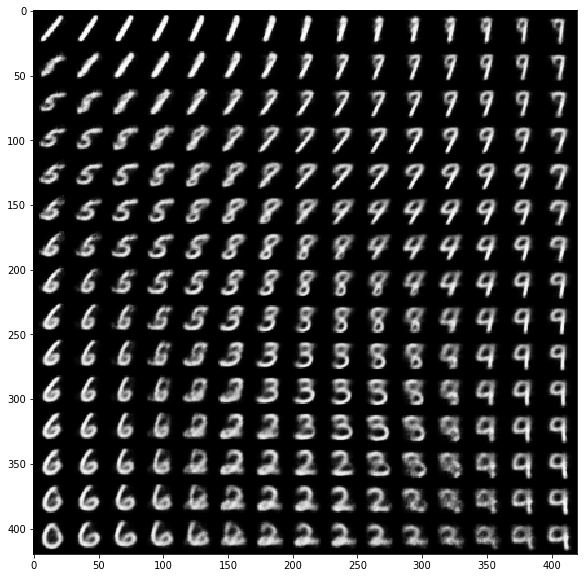
6.从二维潜在空间采样一组点的网络,并将其解码为图像
使用decoder网络将任意潜在空间向量转换为向量
import matplotlib.pyplot as plt
from scipy.stats import norm

# Display a 2D manifold of the digits
n = 15  # figure with 15x15 digits
digit_size = 28
figure = np.zeros((digit_size * n, digit_size * n))
# Linearly spaced coordinates on the unit square were transformed
# through the inverse CDF (ppf) of the Gaussian
# to produce values of the latent variables z,
# since the prior of the latent space is Gaussian
grid_x = norm.ppf(np.linspace(0.05, 0.95, n))
grid_y = norm.ppf(np.linspace(0.05, 0.95, n))

for i, yi in enumerate(grid_x):
    for j, xi in enumerate(grid_y):
        z_sample = np.array([[xi, yi]])
        z_sample = np.tile(z_sample, batch_size).reshape(batch_size, 2)
        x_decoded = decoder.predict(z_sample, batch_size=batch_size)
        digit = x_decoded[0].reshape(digit_size, digit_size)
        figure[i * digit_size: (i + 1) * digit_size,
               j * digit_size: (j + 1) * digit_size] = digit

plt.figure(figsize=(10, 10))
plt.imshow(figure, cmap='Greys_r')
plt.show()
四、搭建 GAN 网络,数据可以是 att_face 和 yaleface
import keras
keras.__version__
Using TensorFlow backend.


'2.3.1'
1.创建生成器
First, we develop a generator model, which turns a vector (from the latent space -- during training it will sampled at random) into a
candidate image. One of the many issues that commonly arise with GANs is that the generator gets stuck with generated images that look like
noise. A possible solution is to use dropout on both the discriminator and generator.
import keras
from keras import layers
import numpy as np

latent_dim = 32
height = 112
width = 92
channels = 1

generator_input = keras.Input(shape=(latent_dim,))

# First, transform the input into a 16x16 128-channels feature map
x = layers.Dense(128 * 56 * 46)(generator_input)
x = layers.LeakyReLU()(x)
x = layers.Reshape((56, 46, 128))(x)

# Then, add a convolution layer
x = layers.Conv2D(256, 5, padding='same')(x)
x = layers.LeakyReLU()(x)

# Upsample to 32x32
x = layers.Conv2DTranspose(256, 4, strides=2, padding='same')(x)
x = layers.LeakyReLU()(x)

# Few more conv layers
x = layers.Conv2D(256, 5, padding='same')(x)
x = layers.LeakyReLU()(x)
x = layers.Conv2D(256, 5, padding='same')(x)
x = layers.LeakyReLU()(x)

# Produce a 32x32 1-channel feature map
x = layers.Conv2D(channels, 7, activation='tanh', padding='same')(x)
generator = keras.models.Model(generator_input, x)
generator.summary()
Model: "model_1"
_________________________________________________________________
Layer (type)                 Output Shape              Param #
=================================================================
input_1 (InputLayer)         (None, 32)                0
_________________________________________________________________
dense_1 (Dense)              (None, 329728)            10881024
_________________________________________________________________
leaky_re_lu_1 (LeakyReLU)    (None, 329728)            0
_________________________________________________________________
reshape_1 (Reshape)          (None, 56, 46, 128)       0
_________________________________________________________________
conv2d_1 (Conv2D)            (None, 56, 46, 256)       819456
_________________________________________________________________
leaky_re_lu_2 (LeakyReLU)    (None, 56, 46, 256)       0
_________________________________________________________________
conv2d_transpose_1 (Conv2DTr (None, 112, 92, 256)      1048832
_________________________________________________________________
leaky_re_lu_3 (LeakyReLU)    (None, 112, 92, 256)      0
_________________________________________________________________
conv2d_2 (Conv2D)            (None, 112, 92, 256)      1638656
_________________________________________________________________
leaky_re_lu_4 (LeakyReLU)    (None, 112, 92, 256)      0
_________________________________________________________________
conv2d_3 (Conv2D)            (None, 112, 92, 256)      1638656
_________________________________________________________________
leaky_re_lu_5 (LeakyReLU)    (None, 112, 92, 256)      0
_________________________________________________________________
conv2d_4 (Conv2D)            (None, 112, 92, 1)        12545
=================================================================
Total params: 16,039,169
Trainable params: 16,039,169
Non-trainable params: 0
_________________________________________________________________
2.创建判别器
Then, we develop a discriminator model, that takes as input a candidate image (real or synthetic) and classifies it into one of two
classes, either "generated image" or "real image that comes from the training set".
discriminator_input = layers.Input(shape=(height, width, channels))
x = layers.Conv2D(128, 3)(discriminator_input)
x = layers.LeakyReLU()(x)
x = layers.Conv2D(128, 4, strides=2)(x)
x = layers.LeakyReLU()(x)
x = layers.Conv2D(128, 4, strides=2)(x)
x = layers.LeakyReLU()(x)
x = layers.Conv2D(128, 4, strides=2)(x)
x = layers.LeakyReLU()(x)
x = layers.Flatten()(x)

# One dropout layer - important trick!
x = layers.Dropout(0.4)(x)

# Classification layer
x = layers.Dense(1, activation='sigmoid')(x)

discriminator = keras.models.Model(discriminator_input, x)
discriminator.summary()

# To stabilize training, we use learning rate decay
# and gradient clipping (by value) in the optimizer.
discriminator_optimizer = keras.optimizers.RMSprop(lr=0.0008, clipvalue=1.0, decay=1e-8)
discriminator.compile(optimizer=discriminator_optimizer, loss='binary_crossentropy')
Model: "model_2"
_________________________________________________________________
Layer (type)                 Output Shape              Param #
=================================================================
input_2 (InputLayer)         (None, 112, 92, 1)        0
_________________________________________________________________
conv2d_5 (Conv2D)            (None, 110, 90, 128)      1280
_________________________________________________________________
leaky_re_lu_6 (LeakyReLU)    (None, 110, 90, 128)      0
_________________________________________________________________
conv2d_6 (Conv2D)            (None, 54, 44, 128)       262272
_________________________________________________________________
leaky_re_lu_7 (LeakyReLU)    (None, 54, 44, 128)       0
_________________________________________________________________
conv2d_7 (Conv2D)            (None, 26, 21, 128)       262272
_________________________________________________________________
leaky_re_lu_8 (LeakyReLU)    (None, 26, 21, 128)       0
_________________________________________________________________
conv2d_8 (Conv2D)            (None, 12, 9, 128)        262272
_________________________________________________________________
leaky_re_lu_9 (LeakyReLU)    (None, 12, 9, 128)        0
_________________________________________________________________
flatten_1 (Flatten)          (None, 13824)             0
_________________________________________________________________
dropout_1 (Dropout)          (None, 13824)             0
_________________________________________________________________
dense_2 (Dense)              (None, 1)                 13825
=================================================================
Total params: 801,921
Trainable params: 801,921
Non-trainable params: 0
_________________________________________________________________
3.对抗网络
Finally, we setup the GAN, which chains the generator and the discriminator. This is the model that, when trained, will move the generator
in a direction that improves its ability to fool the discriminator. This model turns latent space points into a classification decision,
"fake" or "real", and it is meant to be trained with labels that are always "these are real images". So training gan will updates the
weights of generator in a way that makes discriminator more likely to predict "real" when looking at fake images. Very importantly, we
set the discriminator to be frozen during training (non-trainable): its weights will not be updated when training gan. If the
discriminator weights could be updated during this process, then we would be training the discriminator to always predict "real", which is
not what we want!
# Set discriminator weights to non-trainable
# (will only apply to the `gan` model)
discriminator.trainable = False

gan_input = keras.Input(shape=(latent_dim,))
gan_output = discriminator(generator(gan_input))
gan = keras.models.Model(gan_input, gan_output)

gan_optimizer = keras.optimizers.RMSprop(lr=0.0004, clipvalue=1.0, decay=1e-8)
gan.compile(optimizer=gan_optimizer, loss='binary_crossentropy')
4.Gan训练,att_face
att_image = []
att_labels = []

import os
import cv2
from PIL import Image

def read_directory(directory_name):
    for filename in os.listdir(directory_name):
#         print(directory_name+'/'+filename)
        img = Image.open(directory_name+'/'+filename)
        img = np.array(img)
        att_image.append(img)

for i in range(1,41):
    read_directory('face_database/att_face/s'+str(i))
    labels = [i]*10
    att_labels.append(labels)
att_image = np.array(att_image)

att_image.shape
(400, 112, 92)
att_image = att_image.reshape(400,112,92,-1)
att_image.shape
(400, 112, 92, 1)
att_labels = np.array(att_labels)
att_labels = att_labels.reshape(400,1)
att_labels.shape
(400, 1)
import os
from keras.preprocessing import image
# for i in range(1,41):
x_train = att_image[0:10]
#     att_image = att_image[i*10-10:i*10]
x_train = x_train.astype('float32') / 255.
labels = att_labels[0:10]
iterations = 100
batch_size = 5
#     dir_ = '/home/hp40/working/jupyter/DL_sy4/gan_att_face_images/s'+str(i)
#     os.mkdir(dir_)
save_dir = '/home/hp40/working/jupyter/DL_sy4/gan_att_face_images'

    # Start training loop
start = 0
for step in range(iterations):
    # Sample random points in the latent space
    random_latent_vectors = np.random.normal(size=(batch_size, latent_dim))

    # Decode them to fake images
    generated_images = generator.predict(random_latent_vectors)

    # Combine them with real images
    stop = start + batch_size
    real_images = x_train[start: stop]
    combined_images = np.concatenate([generated_images, real_images])

    # Assemble labels discriminating real from fake images
    labels = np.concatenate([np.ones((batch_size, 1)),
                                 np.zeros((batch_size, 1))])
    # Add random noise to the labels - important trick!
    labels += 0.05 * np.random.random(labels.shape)

    # Train the discriminator
    d_loss = discriminator.train_on_batch(combined_images, labels)

    # sample random points in the latent space
    random_latent_vectors = np.random.normal(size=(batch_size, latent_dim))

    # Assemble labels that say "all real images"
    misleading_targets = np.zeros((batch_size, 1))

    # Train the generator (via the gan model,
    # where the discriminator weights are frozen)
    a_loss = gan.train_on_batch(random_latent_vectors, misleading_targets)

    start += batch_size
    if start > len(x_train) - batch_size:
        start = 0

    # Occasionally save / plot
    if step % 10 == 0:
        # Save model weights|
        gan.save_weights('att_face_gan.h5')

        # Print metrics
        print('discriminator loss at step %s: %s' % (step, d_loss))
        print('adversarial loss at step %s: %s' % (step, a_loss))

        # Sve one generated image
        img = image.array_to_img(generated_images[0] * 255., scale=False)
        img.save(os.path.join(save_dir, 'generated_frog' + str(step) + '.png'))

        # Save one real image, for comparison
        img = image.array_to_img(real_images[0] * 255., scale=False)
        img.save(os.path.join(save_dir, 'real_frog' + str(step) + '.png'))
/home/hp40/anaconda3/lib/python3.7/site-packages/keras/engine/training.py:297: UserWarning: Discrepancy between trainable weights and collected trainable weights, did you set `model.trainable` without calling `model.compile` after ?
  'Discrepancy between trainable weights and collected trainable'


discriminator loss at step 0: 0.69491494
adversarial loss at step 0: 0.7011034
discriminator loss at step 10: 0.7188847
adversarial loss at step 10: 0.9296853
discriminator loss at step 20: 0.6825775
adversarial loss at step 20: 0.78894794
discriminator loss at step 30: 0.70663893
adversarial loss at step 30: 1.3348267
discriminator loss at step 40: 0.45972243
adversarial loss at step 40: 0.02316716
discriminator loss at step 50: 0.78936905
adversarial loss at step 50: 0.6956989
discriminator loss at step 60: 0.8633131
adversarial loss at step 60: 4.738366
discriminator loss at step 70: 0.59055054
adversarial loss at step 70: 1.9819958
discriminator loss at step 80: 0.8416172
adversarial loss at step 80: 0.4654118
discriminator loss at step 90: 1.0067852
adversarial loss at step 90: 1.1518466
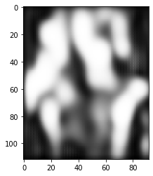
Let's display a few of our fake images:
import matplotlib.pyplot as plt

# Sample random points in the latent space
random_latent_vectors = np.random.normal(size=(10, latent_dim))

# Decode them to fake images
generated_images = generator.predict(random_latent_vectors)

for i in range(generated_images.shape[0]):
    img = image.array_to_img(generated_images[i] * 255., scale=False)
    plt.figure()
    plt.imshow(img,cmap='gray')

plt.show()
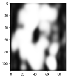
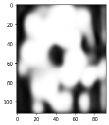
略过一些图片。。。。
5.gan训练,yaleface
yale_labels = []
yale_images = []
import os
import cv2
from PIL import Image
import numpy as np

def read_directory(directory_name):
    for filename in os.listdir(directory_name):
#         print(directory_name+'/'+filename)
        img = Image.open(directory_name+'/'+filename)
        img = np.array(img)
        img = cv2.resize(img,(320,242))
        yale_images.append(img)

read_directory('face_database/yalefaces/yalefaces')
for i in range(1,16):
    if i == 1:
        for i in range(12):
            yale_labels.append(1)
    else:
        for i in range(11):
            yale_labels.append(i)
yale_images = np.array(yale_images)
yale_images.shape
(166, 242, 320)
yale_images = yale_images.reshape(166, 242, 320,-1)
yale_images.shape
(166, 242, 320, 1)
yale_labels = np.array(yale_labels)
yale_labels = yale_labels.reshape(166,1)
yale_labels.shape
(166, 1)
import keras
from keras import layers
import numpy as np

latent_dim = 32
height = 242
width = 320
channels = 1

generator_input = keras.Input(shape=(latent_dim,))

# First, transform the input into a 16x16 128-channels feature map
x = layers.Dense(128 * 121 * 160)(generator_input)
x = layers.LeakyReLU()(x)
x = layers.Reshape((121, 160, 128))(x)

# Then, add a convolution layer
x = layers.Conv2D(256, 5, padding='same')(x)
x = layers.LeakyReLU()(x)

# Upsample to 32x32
x = layers.Conv2DTranspose(256, 4, strides=2, padding='same')(x)
x = layers.LeakyReLU()(x)

# Few more conv layers
x = layers.Conv2D(256, 5, padding='same')(x)
x = layers.LeakyReLU()(x)
x = layers.Conv2D(256, 5, padding='same')(x)
x = layers.LeakyReLU()(x)

# Produce a 32x32 1-channel feature map
x = layers.Conv2D(channels, 7, activation='tanh', padding='same')(x)
generator = keras.models.Model(generator_input, x)
generator.summary()
Model: "model_1"
_________________________________________________________________
Layer (type)                 Output Shape              Param #
=================================================================
input_1 (InputLayer)         (None, 32)                0
_________________________________________________________________
dense_1 (Dense)              (None, 2478080)           81776640
_________________________________________________________________
leaky_re_lu_1 (LeakyReLU)    (None, 2478080)           0
_________________________________________________________________
reshape_1 (Reshape)          (None, 121, 160, 128)     0
_________________________________________________________________
conv2d_1 (Conv2D)            (None, 121, 160, 256)     819456
_________________________________________________________________
leaky_re_lu_2 (LeakyReLU)    (None, 121, 160, 256)     0
_________________________________________________________________
conv2d_transpose_1 (Conv2DTr (None, 242, 320, 256)     1048832
_________________________________________________________________
leaky_re_lu_3 (LeakyReLU)    (None, 242, 320, 256)     0
_________________________________________________________________
conv2d_2 (Conv2D)            (None, 242, 320, 256)     1638656
_________________________________________________________________
leaky_re_lu_4 (LeakyReLU)    (None, 242, 320, 256)     0
_________________________________________________________________
conv2d_3 (Conv2D)            (None, 242, 320, 256)     1638656
_________________________________________________________________
leaky_re_lu_5 (LeakyReLU)    (None, 242, 320, 256)     0
_________________________________________________________________
conv2d_4 (Conv2D)            (None, 242, 320, 1)       12545
=================================================================
Total params: 86,934,785
Trainable params: 86,934,785
Non-trainable params: 0
_________________________________________________________________
discriminator_input = layers.Input(shape=(height, width, channels))
x = layers.Conv2D(128, 3)(discriminator_input)
x = layers.LeakyReLU()(x)
x = layers.Conv2D(128, 4, strides=2)(x)
x = layers.LeakyReLU()(x)
x = layers.Conv2D(128, 4, strides=2)(x)
x = layers.LeakyReLU()(x)
x = layers.Conv2D(128, 4, strides=2)(x)
x = layers.LeakyReLU()(x)
x = layers.Flatten()(x)

# One dropout layer - important trick!
x = layers.Dropout(0.4)(x)

# Classification layer
x = layers.Dense(1, activation='sigmoid')(x)

discriminator = keras.models.Model(discriminator_input, x)
discriminator.summary()

# To stabilize training, we use learning rate decay
# and gradient clipping (by value) in the optimizer.
discriminator_optimizer = keras.optimizers.RMSprop(lr=0.0008, clipvalue=1.0, decay=1e-8)
discriminator.compile(optimizer=discriminator_optimizer, loss='binary_crossentropy')
Model: "model_2"
_________________________________________________________________
Layer (type)                 Output Shape              Param #
=================================================================
input_2 (InputLayer)         (None, 242, 320, 1)       0
_________________________________________________________________
conv2d_5 (Conv2D)            (None, 240, 318, 128)     1280
_________________________________________________________________
leaky_re_lu_6 (LeakyReLU)    (None, 240, 318, 128)     0
_________________________________________________________________
conv2d_6 (Conv2D)            (None, 119, 158, 128)     262272
_________________________________________________________________
leaky_re_lu_7 (LeakyReLU)    (None, 119, 158, 128)     0
_________________________________________________________________
conv2d_7 (Conv2D)            (None, 58, 78, 128)       262272
_________________________________________________________________
leaky_re_lu_8 (LeakyReLU)    (None, 58, 78, 128)       0
_________________________________________________________________
conv2d_8 (Conv2D)            (None, 28, 38, 128)       262272
_________________________________________________________________
leaky_re_lu_9 (LeakyReLU)    (None, 28, 38, 128)       0
_________________________________________________________________
flatten_1 (Flatten)          (None, 136192)            0
_________________________________________________________________
dropout_1 (Dropout)          (None, 136192)            0
_________________________________________________________________
dense_2 (Dense)              (None, 1)                 136193
=================================================================
Total params: 924,289
Trainable params: 924,289
Non-trainable params: 0
_________________________________________________________________
# Set discriminator weights to non-trainable
# (will only apply to the `gan` model)
discriminator.trainable = False

gan_input = keras.Input(shape=(latent_dim,))
gan_output = discriminator(generator(gan_input))
gan = keras.models.Model(gan_input, gan_output)

gan_optimizer = keras.optimizers.RMSprop(lr=0.0004, clipvalue=1.0, decay=1e-8)
gan.compile(optimizer=gan_optimizer, loss='binary_crossentropy')
import os
from keras.preprocessing import image
# for i in range(1,41):
x_train = yale_images[0:12]
#     att_image = att_image[i*10-10:i*10]
x_train = x_train.astype('float32') / 255.
labels = yale_labels[0:12]
iterations = 100
batch_size = 5
#     dir_ = '/home/hp40/working/jupyter/DL_sy4/gan_att_face_images/s'+str(i)
#     os.mkdir(dir_)
save_dir = '/home/hp40/working/jupyter/DL_sy4/gan_yale_face_images'

    # Start training loop
start = 0
for step in range(iterations):
    # Sample random points in the latent space
    random_latent_vectors = np.random.normal(size=(batch_size, latent_dim))

    # Decode them to fake images
    generated_images = generator.predict(random_latent_vectors)

    # Combine them with real images
    stop = start + batch_size
    real_images = x_train[start: stop]
    combined_images = np.concatenate([generated_images, real_images])

    # Assemble labels discriminating real from fake images
    labels = np.concatenate([np.ones((batch_size, 1)),
                                 np.zeros((batch_size, 1))])
    # Add random noise to the labels - important trick!
    labels += 0.05 * np.random.random(labels.shape)

    # Train the discriminator
    d_loss = discriminator.train_on_batch(combined_images, labels)

    # sample random points in the latent space
    random_latent_vectors = np.random.normal(size=(batch_size, latent_dim))

    # Assemble labels that say "all real images"
    misleading_targets = np.zeros((batch_size, 1))

    # Train the generator (via the gan model,
    # where the discriminator weights are frozen)
    a_loss = gan.train_on_batch(random_latent_vectors, misleading_targets)

    start += batch_size
    if start > len(x_train) - batch_size:
        start = 0

    # Occasionally save / plot
    if step % 10 == 0:
        # Save model weights|
        gan.save_weights('yale_faces_gan.h5')

        # Print metrics
        print('discriminator loss at step %s: %s' % (step, d_loss))
        print('adversarial loss at step %s: %s' % (step, a_loss))

        # Sve one generated image
        img = image.array_to_img(generated_images[0] * 255., scale=False)
        img.save(os.path.join(save_dir, 'generated_frog' + str(step) + '.png'))

        # Save one real image, for comparison
        img = image.array_to_img(real_images[0] * 255., scale=False)
        img.save(os.path.join(save_dir, 'real_frog' + str(step) + '.png'))
/home/hp40/anaconda3/lib/python3.7/site-packages/keras/engine/training.py:297: UserWarning: Discrepancy between trainable weights and collected trainable weights, did you set `model.trainable` without calling `model.compile` after ?
  'Discrepancy between trainable weights and collected trainable'


discriminator loss at step 0: 0.6982208
adversarial loss at step 0: 0.6396512
discriminator loss at step 10: 0.9123316
adversarial loss at step 10: 14.80499
discriminator loss at step 20: 0.46674195
adversarial loss at step 20: 1.5911399
discriminator loss at step 30: 0.24239938
adversarial loss at step 30: 1.848883
discriminator loss at step 40: 1.4674227
adversarial loss at step 40: 1.7690643
discriminator loss at step 50: 0.48709828
adversarial loss at step 50: 2.509427