Deep learning with Python 学习笔记（1）

深度学习基础

Python 的 Keras 库来学习手写数字分类，将手写数字的灰度图像(28 像素 ×28 像素)划分到 10 个类别
中(0~9)
神经网络的核心组件是层(layer),它是一种数据处理模块，它从输入数据中提取表示，紧接着的一个例子中，将含有两个Dense 层,它们是密集连接(也叫全连接)的神经层，最后是一个10路的softmax层，它将返回一个由 10 个概率值(总和为 1)组成的数组。每个概率值表示当前数字图像属于 10 个数字类别中某一个的概率
损失函数(loss function):网络如何衡量在训练数据上的性能,即网络如何朝着正确的方向前进
优化器(optimizer):基于训练数据和损失函数来更新网络的机制

from keras.datasets import mnist
from keras import models
from keras import layers
from keras.utils import to_categorical


# 加载数据
(train_images, train_labels), (test_images, test_labels) = mnist.load_data()
print("训练图片个数与尺寸： ", train_images.shape, "标签数： ", len(train_labels))
print("测试图片数量与尺寸： ", test_images.shape, "标签数： ", len(test_labels))
# 网络架构
network = models.Sequential()
network.add(layers.Dense(512, activation='relu', input_shape=(28 * 28,)))
network.add(layers.Dense(10, activation="softmax"))
# 编译
network.compile(optimizer='rmsprop', loss='categorical_crossentropy', metrics=['accuracy'])
# 数据预处理,将其变换为网络要求的形状，并缩放到所有值都在 [0, 1] 区间
train_images = train_images.reshape((60000, 28 * 28))
train_images = train_images.astype('float32') / 255
test_images = test_images.reshape((10000, 28 * 28))
test_images = test_images.astype('float32') / 255
# 对标签进行分类编码
train_labels = to_categorical(train_labels)
test_labels = to_categorical(test_labels)
# 训练模型，epochs表示训练遍数，batch_size表示每次喂给网络的数据数目
network.fit(train_images, train_labels, epochs=5, batch_size=128)
# 检测在测试集上的正确率
test_loss, test_acc = network.evaluate(test_images, test_labels)
print('正确率: ', test_acc)

张量是矩阵向任意维度的推广，仅包含一个数字的张量叫作标量，数字组成的数组叫作向量(vector)或一维张量(1D 张量)。一维张量只有一个轴
显示数字图片

(train_images, train_labels), (test_images, test_labels) = mnist.load_data("/home/fan/dataset/mnist.npz")
# 显示第0个数字
import matplotlib.pyplot as plt
digit = train_images[0]
plt.imshow(digit, cmap=plt.cm.binary)
plt.show()

一些数据张量
向量数据: 2D 张量,形状为 (samples, features)
时间序列数据或序列数据: 3D 张量,形状为 (samples, timesteps, features)
图像: 4D 张量,形状为 (samples, height, width, channels) 或 (samples, channels, height, width)
视频: 5D 张量,形状为 (samples, frames, height, width, channels) 或 (samples, frames, channels, height, width)

当时间(或序列顺序)对于数据很重要时,应该将数据存储在带有时间轴的 3D 张量中

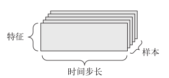
根据惯例,时间轴始终是第 2 个轴
图像通常具有三个维度: 高度、宽度和颜色深度
灰度图像只有一个颜色通道,因此可以保存在 2D 张量中
4D张量表示

图像张量的形状有两种约定: 通道在后(channels-last)的约定(在 TensorFlow 中使用)和通道在前(channels-first)的约定(在 Theano 中使用)。TensorFlow 机器学习框架将颜色深度轴放在最后: (samples, height, width, color_depth)，Theano将图像深度轴放在批量轴之后: (samples, color_depth, height, width)，Keras 框架同时支持这两种格式
视频数据为 5D 张量，每一帧都可以保存在一个形状为 (height, width, color_depth) 的 3D 张量中,因此一系列帧可以保存在一个形状为 (frames, height, width, color_depth) 的 4D 张量中,而不同视频组成的批量则可以保存在一个 5D 张量中,其形状为(samples, frames, height, width, color_depth)
一个以每秒 4 帧采样的 60 秒 YouTube 视频片段,视频尺寸为 144×256,这个视频共有 240 帧。4 个这样的视频片段组成的批量将保存在形状为 (4, 240, 144, 256, 3)的张量中

如果将两个形状不同的张量相加，较小的张量会被广播(broadcast),以匹配较大张量的形状：

1. 向较小的张量添加轴(叫作广播轴)，使其 ndim 与较大的张量相同
2. 将较小的张量沿着新轴重复，使其形状与较大的张量相同

a = np.array([[2, 2], [1, 1]])
c = np.array([3, 3])
print(a + c)

结果为

[[5 5]  
 [4 4]]

如果一个张量的形状是 (a, b, ... n, n+1, ... m) ,另一个张量的形状是 (n, n+1, ... m) ,那么你通常可以利用广播对它们做两个张量之间的逐元素运算。广播操作会自动应用于从 a 到 n-1 的轴

在 Numpy、Keras、Theano 和 TensorFlow 中,都是用 * 实现逐元素乘积，在 Numpy 和 Keras 中,都是用标准的 dot 运算符来实现点积

a = np.array([1, 2])
b = np.array([[5], [6]])
# 输出[17]
print(a.dot(b))

张量变形是指改变张量的行和列,以得到想要的形状。变形后的张量的元素总个数与初始张量相同

a = np.array([[0, 1], [2, 3], [4, 5]])
print(a)
print("after reshape: \n", a.reshape((2, 3)))

输出

[[0 1]
 [2 3]
 [4 5]]
after reshape: 
 [[0 1 2]
 [3 4 5]]

转置 np.transpose(x)

SGD(stochastic gradient descent) -- 随机梯度下降

不同的张量格式与不同的数据处理类型需要用到不同的层，简单的向量数据保存在形状为 (samples, features) 的 2D 张量中,通常用密集连接层[densely connected layer，也叫全连接层(fully connected layer)或密集层(dense layer)，对应于 Keras 的 Dense 类]来处理。序列数据保存在形状为 (samples, timesteps, features) 的 3D 张量中，通常用循环层(recurrent layer，比如 Keras 的 LSTM 层)来处理。图像数据保存在 4D 张量中，通常用二维卷积层(Keras 的 Conv2D )来处理

Keras框架具有层兼容性，具体指的是每一层只接受特定形状的输入张量,并返回特定形状的输出张量

layer = layers.Dense(32, input_shape=(784,))

创建了一个层,只接受第一个维度大小为 784 的 2D 张量作为输入。这个层将返回一个张量,第一个维度的大小变成了 32 因此，这个层后面只能连接一个接受 32 维向量作为输入的层，使用 Keras 时，你无须担心兼容性，因为向模型中添加的层都会自动匹配输入层的形状，下一次层可以写为

model.add(layers.Dense(32))

它可以自动推导出输入形状等于上一层的输出形状

具有多个输出的神经网络可能具有多个损失函数(每个输出对应一个损失函数)。但是，梯度下降过程必须基于单个标量损失值。因此，对于具有多个损失函数的网络，需要将所有损失函数取平均，变为一个标量值

一个 Keras 工作流程

1. 定义训练数据: 输入张量和目标张量
2. 定义层组成的网络(或模型),将输入映射到目标
3. 配置学习过程:选择损失函数、优化器和需要监控的指标
4. 调用模型的 fit 方法在训练数据上进行迭代

定义模型有两种方法:
一种是使用 Sequential 类(仅用于层的线性堆叠,这是目前最常见的网络架构)
另一种是函数式 API(functional API，用于层组成的有向无环图，让你可以构建任意形式的架构)
Sequential 类定义两层模型

model = models.Sequential()
model.add(layers.Dense(32, activation='relu', input_shape=(784,)))
model.add(layers.Dense(10, activation='softmax'))

函数式 API 定义的相同模型

input_tensor = layers.Input(shape=(784,))
x = layers.Dense(32, activation='relu')(input_tensor)
output_tensor = layers.Dense(10, activation='softmax')(x)
model = models.Model(inputs=input_tensor, outputs=output_tensor)

以下学习根据电影评论的文字内容将其划分为正面或负面
使用 IMDB 数据集，数据集被分为用于训练的 25 000 条评论与用于测试的 25 000 条评论,训练集和测试集都包含 50% 的正面评论和 50% 的负面评论
其中，数据集中的labels 都是 0 和 1 组成的列表，0代表负面(negative)，1 代表正面(positive)
你不能将整数序列直接输入神经网络。你需要将列表转换为张量。转换方法有以下两种

1. 填充列表，使其具有相同的长度，再将列表转换成形状为 (samples, word_indices)的整数张量，然后网络第一层使用能处理这种整数张量的层
2. 对列表进行 one-hot 编码,将其转换为 0 和 1 组成的向量。举个例子，序列 [3, 5] 将会被转换为 10 000 维向量，只有索引为 3 和 5 的元素是 1，其余元素都是 0，然后网络第一层可以用 Dense 层，它能够处理浮点数向量数据

训练代码

from keras.datasets import imdb
import os
import numpy as np
from keras import models
from keras import layers
import matplotlib.pyplot as plt


# 将整数序列编码为二进制矩阵
def vectorize_sequences(sequences, dimension=10000):
    results = np.zeros((len(sequences), dimension))
    for i, sequence in enumerate(sequences):
        # results[i] 的指定索引设为 1
        results[i, sequence] = 1
    return results


data_url_base = "/home/fan/dataset"
# 下载数据且只保留出现频率最高的前10000个单词
(train_data, train_labels), (test_data, test_labels) = imdb.load_data(num_words=10000, path=os.path.join(data_url_base, "imdb.npz"))

# 将某条评论迅速解码为英文单词
# word_index 是一个将单词映射为整数索引的字典
word_index = imdb.get_word_index(path=os.path.join(data_url_base, "imdb_word_index.json"))
# 将整数索引映射为单词
reverse_word_index = dict([(value, key) for (key, value) in word_index.items()])
# 索引减去了 3,因为 0、1、2是为“padding”(填充)、
# “start of sequence”(序列开始)、“unknown”(未知词)分别保留的索引
decoded_review = ' '.join([reverse_word_index.get(i - 3, '?') for i in train_data[0]])
print(decoded_review)

# 将数据向量化
x_train = vectorize_sequences(train_data)
x_test = vectorize_sequences(test_data)
# 将标签向量化
y_train = np.asarray(train_labels).astype('float32')
y_test = np.asarray(test_labels).astype('float32')

# 设计网络
# 两个中间层,每层都有 16 个隐藏单元
# 第三层输出一个标量,预测当前评论的情感
# 中间层使用 relu 作为激活函数,最后一层使用 sigmoid 激活以输出一个 0~1 范围内的概率值
model = models.Sequential()
model.add(layers.Dense(16, activation='relu', input_shape=(10000,)))
model.add(layers.Dense(16, activation='relu'))
model.add(layers.Dense(1, activation='sigmoid'))
# 模型编译
# binary_crossentropy二元交叉熵
model.compile(optimizer='rmsprop', loss='binary_crossentropy', metrics=['acc'])
# 留出验证集
x_val = x_train[:10000]
partial_x_train = x_train[10000:]
y_val = y_train[:10000]
partial_y_train = y_train[10000:]
history = model.fit(partial_x_train, partial_y_train, epochs=20, batch_size=512, validation_data=(x_val, y_val))
# 得到训练过程中的所有数据
history_dict = history.history
print(history_dict.keys())

# 绘制训练损失和验证损失
loss_values = history_dict['loss']
val_loss_values = history_dict['val_loss']
epochs = range(1, len(loss_values) + 1)
# 'bo' 蓝色圆点
plt.plot(epochs, loss_values, 'bo', label='Training loss')
# 'b' 蓝色实线
plt.plot(epochs, val_loss_values, 'b', label='Validation loss')
plt.title("Training and Validation loss")
plt.xlabel('Epochs')
plt.legend()
plt.show()

# 绘制训练精度和验证精度
# plt.clf() 清空图像
acc = history_dict['acc']
val_acc = history_dict['val_acc']

plt.plot(epochs, acc, 'bo', label='Training acc')
plt.plot(epochs, val_acc, 'b', label='Validation acc')
plt.title('Training and validation accuracy')
plt.xlabel('Epochs')
plt.ylabel('Accuracy')
plt.legend()
plt.show()

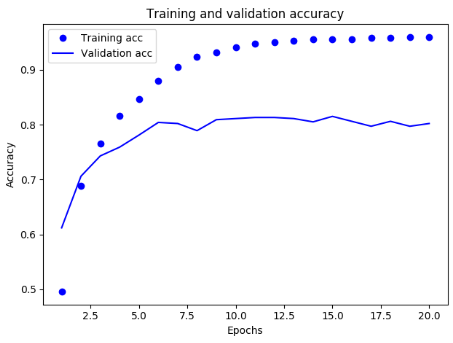
结果如下

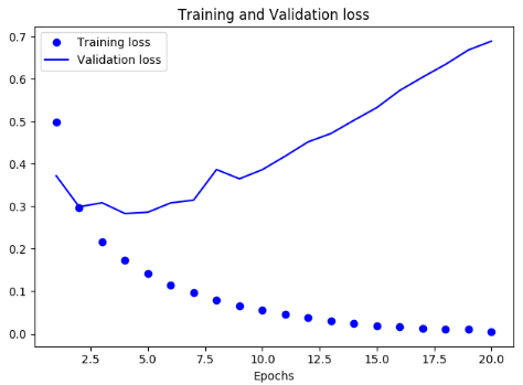
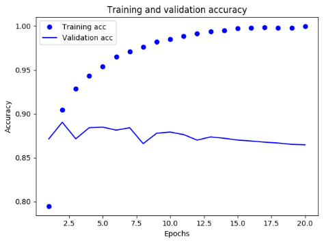
可见训练损失每轮都在降低，训练精度每轮都在提升，但验证损失和验证精度并非如此，这是因为我们遇到了过拟合的情况，可以采用多种方法防止过拟合，如增加数据样本，减少训练次数，减少网络参数等
使用训练好的网络对新数据进行预测

model.predict(x_test)

多分类问题 -- 新闻主题分类
如果每个数据点只能划分到一个类别，那么这就是一个单标签、多分类问题，而如果每个数据点可以划分到多个类别(主题)，那它就是一个多标签、多分类问题，此处为单标签、多分类问题

将标签向量化有两种方法

1. 你可以将标签列表转换为整数张量
2. 或者使用 one-hot 编码，one-hot 编码是分类数据广泛使用的一种格式，也叫分类编码(categorical encoding)

将标签转换为整数张量

y_train = np.array(train_labels)
y_test = np.array(test_labels)

对于此种编码方法，我们选择的损失函数应该为sparse_categorical_crossentropy，该编码方法适用于整数标签

新闻分类示例

from keras.datasets import reuters
import numpy as np
from keras.utils.np_utils import to_categorical
from keras import models
from keras import layers
import matplotlib.pyplot as plt


# 将整数序列编码为二进制矩阵
def vectorize_sequences(sequences, dimension=10000):
    results = np.zeros((len(sequences), dimension))
    for i, sequence in enumerate(sequences):
        # results[i] 的指定索引设为 1
        results[i, sequence] = 1
    return results


# 将数据限定为前10000个最常出现的单词
(train_data, train_labels), (test_data, test_labels) = reuters.load_data(num_words=10000, path="/home/fan/dataset/reuters/reuters.npz")
# 新闻解析
word_index = reuters.get_word_index(path="/home/fan/dataset/reuters/reuters_word_index.json")
reversed_word_index = dict([(value, key) for (key, value) in word_index.items()])
# 索引减去了3，因为 0、1、2 是为“padding”( 填 充 )、“start of
# sequence”(序列开始)、“unknown”(未知词)分别保留的索引
decoded_newswire = ' '.join([reversed_word_index.get(i-3, '?') for i in train_data[0]])
print(decoded_newswire)
# 标签的索引范围为0 - 45
print(np.amax(train_labels))

# 数据向量化
x_train = vectorize_sequences(train_data)
x_test = vectorize_sequences(test_data)
# 标签向量化
one_hot_train_labels = to_categorical(train_labels)
one_hot_test_labels = to_categorical(test_labels)

model = models.Sequential()
model.add(layers.Dense(64, activation='relu', input_shape=(10000, )))
model.add(layers.Dense(64, activation='relu'))
model.add(layers.Dense(46, activation='softmax'))

model.compile(optimizer='rmsprop', loss='categorical_crossentropy', metrics=['accuracy'])
# 留出1000验证集
x_val = x_train[:1000]
partial_x_train = x_train[1000:]
y_val = one_hot_train_labels[:1000]
partial_y_train = one_hot_train_labels[1000:]

history = model.fit(partial_x_train, partial_y_train, epochs=20, batch_size=512, validation_data=(x_val, y_val))

loss = history.history['loss']
val_loss = history.history['val_loss']
epochs = range(1, len(loss) + 1)
plt.plot(epochs, loss, 'bo', label='Training loss')
plt.plot(epochs, val_loss, 'b', label='Validation loss')
plt.title('Training and validation loss')
plt.xlabel('Epochs')
plt.ylabel('Loss')
plt.legend()
plt.show()

acc = history.history['acc']
val_acc = history.history['val_acc']
plt.plot(epochs, acc, 'bo', label='Training acc')
plt.plot(epochs, val_acc, 'b', label='Validation acc')
plt.title('Training and validation accuracy')
plt.xlabel('Epochs')
plt.ylabel('Accuracy')
plt.legend()
plt.show()

实验结果
Loss

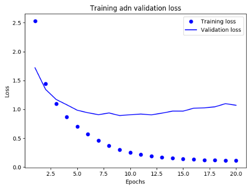
Accuracy

要点

1. 如果要对 N 个类别的数据点进行分类，网络的最后一层应该是大小为 N 的 Dense 层
2. 对于单标签、多分类问题，网络的最后一层应该使用 softmax 激活,这样可以输出在 N 个输出类别上的概率分布

回归问题 预测一个连续值而不是离散的标签
当我们将取值范围差异很大的数据输入到神经网络中，网络可能会自动适应这种数据，但是学习肯定是困难的。对于这种数据，普遍采用的最佳实践是对每个特征做标准化，即对于输入数据的每个特征(输入数据矩阵中的列)，减去特征平均值，再除以标准差，这样得到的特征平均值为 0，标准差为 1
此处要注意，用于测试数据标准化的均值和标准差都是在训练数据上计算得到的。在工作流程中，你不能使用在测试数据上计算得到的任何结果，即使是像数据标准化这么简单的事情也不行
当样本数量很少，我们应该使用一个非常小的网络，不然会出现严重的过拟合
当进行标量回归时，网络的最后一层只设置一个单元，不需要激活，是一个线性层，添加激活函数将会限制输出范围
当你的数据量较小时，无法给验证集分出较大的样本，这导致验证集的划分方式会造成验证分数上有很大的方差，而无法对模型进行有效的评估，这时我们可以选用K折交叉验证
K折交叉验证

例子

from keras.datasets import boston_housing
from keras import models
from keras import layers
import numpy as np
import matplotlib.pyplot as plt


def builde_model():
    model = models.Sequential()
    model.add(layers.Dense(64, activation='relu',
                           input_shape=(train_data.shape[1],)))
    model.add(layers.Dense(64, activation='relu'))
    model.add(layers.Dense(1))
    model.compile(optimizer='rmsprop', loss='mse', metrics=['mae'])
    return model


(train_data, train_targets), (test_data, test_targets) = boston_housing.load_data('/home/fan/dataset/boston_housing.npz')
# 数据标准化
mean = train_data.mean(axis=0)
train_data -= mean
std = train_data.std(axis=0)
train_data /= std
test_data -= mean
test_data /= std

k = 4
num_val_samples = len(train_data)
num_epochs = 500
all_mae_histories = []
for i in range(k):
    print('processing fold #', i)
    val_data = train_data[i * num_val_samples: (i + 1) * num_val_samples]
    val_targets = train_targets[i * num_val_samples: (i + 1) * num_val_samples]
    partial_train_data = np.concatenate([train_data[:i * num_val_samples], train_data[(i + 1) * num_val_samples:]], axis=0)
    partial_train_targets = np.concatenate([train_targets[:i * num_val_samples], train_targets[(i + 1) * num_val_samples:]], axis=0)

    model = builde_model()
    # 静默模式 verbose = 0
    history = model.fit(partial_train_data, partial_train_targets, validation_data=(val_data, val_targets), epochs=num_epochs, batch_size=1, verbose=0)
    print(history.history.keys())
    if 'mean_absolute_error' not in history.history.keys():
        continue
    mae_history = history.history['mean_absolute_error']
    all_mae_histories.append(mae_history)
average_mae_history = [np.mean([x[i] for x in all_mae_histories]) for i in range(num_epochs)]


def smooth_curve(points, factor=0.9):
    smoothed_points = []
    for point in points:
        if smoothed_points:
            previous = smoothed_points[-1]
            smoothed_points.append(previous * factor + point * (1 - factor))
        else:
            smoothed_points.append(point)
    return smoothed_points


smooth_mae_history = smooth_curve(average_mae_history[10:])
plt.plot(range(1, len(smooth_mae_history) + 1), smooth_mae_history)
plt.xlabel('Epochs')
plt.ylabel('Validation mae')
plt.show()

实验结果
每个数据点为前面数据点的指数移动平均值

机器学习的四个分支

1. 监督学习 给定一组样本(通常由人工标注)，它可以学会将输入数据映射到已知目标，如

分类
回归
序列生成 给定一张图像，预测描述图像的文字
语法树预测 给定一个句子，预测其分解生成的语法树
目标检测 给定一张图像，在图中特定目标的周围画一个边界框
图像分割 给定一张图像，在特定物体上画一个像素级的掩模

2. 无监督学习 在没有目标的情况下寻找输入数据的有趣变换，其目的在于数据可视化、数据压缩、数据去噪或更好地理解数据中的相关性，如

降维
聚类

3. 自监督学习 是没有人工标注的标签的监督学习，标签仍然存在，但它们是从输入数据中生成的，通常是使用启发式算法生成的，如

自编码器其生成的目标就是未经修改的输入
给定视频中过去的帧来预测下一帧或者给定文本中前面的词来预测下一个词(用未来的输入数据作为监督)

4. 强化学习

在强化学习中，智能体(agent)接收有关其环境的信息，并学会选择使某种奖励最大化的行动

机器学习的目的是得到可以泛化(generalize)的模型，即在前所未见的数据上表现很好的模型，而过拟合则是核心难点
评估模型的重点是将数据划分为三个集合: 训练集、验证集和测试集
划分为这三个集合的原因是：
训练集用来训练网络中的参数，验证集用来调节网络超参数，测试集用来测试网络性能，需要注意的是我们不应该使用模型读取任何测试集相关的信息然后依此来调节模型

如果可用的数据相对较少，而你又需要尽可能精确地评估模型，那么可以选择带有打乱数据的重复 K 折验证(iterated K-fold validation with shuffling)
具体做法：多次使用 K 折验证，在每次将数据划分为 K 个分区之前都先将数据打乱。最终分数是每次 K 折验证分数的平均值，这种方法一共要训练和评估 P×K 个模型，计算代价很大

选择模型评估方法时，需要注意以下几点：

1. 数据代表性

训练的数据要能够代表整体，这时应该将数据打乱

2. 时间箭头

当数据包含数据信息时，应该始终确保测试集中所有数据的时间都晚于训练集数据

3. 数据冗余

当存在数据冗余时，打乱数据可能会造成训练集和验证集出现重复的数据，而我们要确保训练集和验证集之间没有交集

将数据输入神经网络之前，一般我们都需要进行数据预处理，以使其与我们模型需要输入类型相匹配，包括

1. 向量化

神经网络的所有输入和目标都必须是浮点数张量

2. 值标准化

输入数据应该具有以下特征
取值较小: 大部分值都应该在 0~1 范围内
同质性(homogenous): 所有特征的取值都应该在大致相同的范围内
一种更严格的标准化为将： 每个特征分别标准化，使其均值为 0，标准差为 1

3. 处理缺失值

一般来说，对于神经网络，将缺失值设置为 0 是安全的，只要 0 不是一个有意义的值。网络能够从数据中学到 0 意味着缺失数据，并且会忽略这个值
但是当网络在没有缺失值的情况下训练，这时候网络就不能学会忽略缺失值，这时我们需要人为生成一些有缺失项的训练样本

特征工程(feature engineering)是指将数据输入模型之前，利用你自己关于数据和机器学习算法(这里指神经网络)的知识对数据进行硬编码的变换(不是模型学到的)，以改善模型的效果
良好的特征可以让你用更少的数据、更少的资源、更优雅地解决问题

优化(optimization)是指调节模型以在训练数据上得到最佳性能(即机器学习中的学习)，而泛化(generalization)是指训练好的模型在前所未见的数据上的性能好坏。机器学习的目的当然是得到良好的泛化
训练开始时，优化和泛化是相关的: 训练数据上的损失越小，测试数据上的损失也越小。这时的模型是欠拟合(underfit)的，即仍有改进的空间，网络还没有对训练数据中所有相关模式建模；但在训练数据上迭代一定次数之后，泛化不再提高，验证指标先是不变，然后开始变差，即模型开始过拟合。这时模型开始学习仅和训练数据有关的模式，但这种模式对新数据来说是错误的或无关紧要的
防止过拟合的方法：

1. 获取更多的训练数据
2. 减小网络大小

防止过拟合的最简单的方法就是减小模型大小，即减少模型中可学习参数的个数
要找到合适的模型大小，一般的工作流程是开始时选择相对较少的层和参数，然后逐渐增加层的大小或增加新层，直到这种增加对验证损失的影响变得很小

3. 添加权重正则化

理论：简单模型比复杂模型更不容易过拟合
此处简单模型指参数值分布的熵更小的模型或参数更少的模型
方法：强制让模型权重只能取较小的值，从而限制模型的复杂度
如 L_p正则化
L1 正则化(L1 regularization):添加的成本与权重系数的绝对值成正比
L2 正则化(L2 regularization):添加的成本与权重系数的平方成正比

4. 添加 dropout 正则化

训练过程中随机将该层的一些输出特征舍弃

Keras添加正则化的方式

model.add(layers.Dense(16, kernel_regularizer=regularizers.l2(0.001), activation='relu', input_shape=(10000,)))

其中0.001为正则化损失系数
由于这个惩罚项只在训练时添加，所以这个网络的训练损失会比测试损失大很多

如果使用dropout正则化的话，dropout 比率(dropout rate)是被设为 0 的特征所占的比例，通常在 0.2~0.5范围内。测试时没有单元被舍弃，而该层的输出值需要按 dropout 比率缩小，因为这时比训练时有更多的单元被激活，需要加以平衡
在 Keras 中，你可以通过 Dropout 层向网络中引入 dropout，dropout 将被应用于前面一层的输出

model.add(layers.Dropout(0.5))

常用的由问题类型选择的最后一层激活和损失函数

问题类型	最后一层激活	损失函数
二分类问题	sigmoid	binary_crossentropy
多分类、单标签问题	softmax	categorical_crossentropy
多分类、多标签问题	sigmoid	binary_crossentropy
回归到任意值	无	mse
回归到 0~1 范围内的值	sigmoid	mse 或 binary_crossentropy

在模型确认之后，我们需要优化我们的网络以达到最佳的性能，此时可以尝试以下几项：

1. 添加 dropout
2. 尝试不同的架构:增加或减少层数
3. 添加 L1 和 / 或 L2 正则化
4. 尝试不同的超参数(比如每层的单元个数或优化器的学习率),以找到最佳配置
5. (可选)反复做特征工程:添加新特征或删除没有信息量的特征

Deep learning with Python 学习笔记（2）