【数据分析与科学计算可视化】numpy 和 matplotlib库总结

一、numpy库

numpy：科学计算包，支持N维数组运算、处理大型矩阵、成熟的广播函数库、矢量运算、线性代数、傅里叶变换、随机数生成，并可与C++/Fortran语言无缝结合。树莓派Python v3默认安装已经包含了numpy。

另：scipy：scipy依赖于numpy，提供了更多的数学工具，包括矩阵运算、线性方程组求解、积分、优化、插值、信号处理、图像处理、统计等等。

1.扩展库numpy简介

导入模板：(交换式)

 >>>import numpy as np

2.numpy库应用于数组

(1)简单数组的生成

>>>import numpy as np   #把列表转化为数组
>>> np.array([0,1,2,3,4])
array([0, 1, 2, 3, 4])

>>>np.array((0,1,2,3,4))   # 元组转化为数组
array([0, 1, 2, 3, 4])

  >>>np.array(range(5))     # 把range对象转换成数组
  array([0, 1, 2, 3, 4])  

  >>>np.array([[1,2,3,4,],[5,6,7,8]])  #二维数组
  array([[1, 2, 3, 4],
        [5, 6, 7, 8]])

  >>>np.arange(8)   # 类似于内置函数range()

  array([0,1,2,3,4,5,6,7])

  >>>np.arange(1,10,1)   #以步长为二的数组
  array([1, 2, 3, 4, 5, 6, 7, 8, 9])

>>> np.linspace(0, 10, 11)         # 等差数组，包含11个数
array([  0.,   1.,   2.,   3.,   4.,   5.,   6.,   7.,   8.,   9.,  10.])

>>> np.linspace(0, 10, 11, endpoint=False) # 不包含终点
array([ 0.        ,  0.90909091,  1.81818182,  2.72727273,  3.63636364,
        4.54545455,  5.45454545,  6.36363636,  7.27272727,  8.18181818,
        9.09090909])

>>> np.logspace(0, 100, 10)        # 对数数组
array([ 1.00000000e+000,   1.29154967e+011,   1.66810054e+022,
        2.15443469e+033,   2.78255940e+044,   3.59381366e+055,
        4.64158883e+066,   5.99484250e+077,   7.74263683e+088,
        1.00000000e+100])

>>> np.logspace(1,6,5, base=2)     # 对数数组，相当于2 ** np.linspace(1,6,5)
array([  2.        ,   4.75682846,  11.3137085 ,  26.90868529,  64.        ])

>>> np.zeros(3)                    # 全0一维数组
array([ 0.,  0.,  0.])

>>> np.ones(3)                     # 全1一维数组
array([ 1.,  1.,  1.])

（2）0,1数组、单位矩阵的生成

>>> np.zeros((3,3))              # 全0二维数组，3行3列
[[ 0.  0.  0.]
 [ 0.  0.  0.]
 [ 0.  0.  0.]]

>>> np.zeros((3,1))              # 全0二维数组，3行1列
array([[ 0.],
       [ 0.],
       [ 0.]])

>>> np.zeros((1,3))              # 全0二维数组，1行3列
array([[ 0.,  0.,  0.]])

>>> np.ones((1,3))               # 全1二维数组
array([[ 1.,  1.,  1.]])

>>> np.ones((3,3))               # 全1二维数组
array([[ 1.,  1.,  1.],
       [ 1.,  1.,  1.],
       [ 1.,  1.,  1.]])

>>> np.identity(3)      # 单位矩阵
array([[ 1.,  0.,  0.],
       [ 0.,  1.,  0.],
       [ 0.,  0.,  1.]])

>>> np.identity(2)
array([[ 1.,  0.],
       [ 0.,  1.]])

>>> np.empty((3,3))     # 空数组，只申请空间而不初始化，元素值是不确定的
array([[ 0.,  0.,  0.],
       [ 0.,  0.,  0.],
       [ 0.,  0.,  0.]])

（3）数组与数值的简单运算

>>> x = np.array((1, 2, 3, 4, 5))    # 创建数组对象
>>> x
array([1, 2, 3, 4, 5])

>>> x * 2                            # 数组与数值相乘，返回新数组
array([ 2, 4, 6, 8, 10])

>>> x / 2                            # 数组与数值相除
array([ 0.5, 1. , 1.5, 2. , 2.5])

>>> x // 2                           # 数组与数值整除
array([0, 1, 1, 2, 2], dtype=int32)

>>> x ** 3                           # 幂运算
array([1, 8, 27, 64, 125], dtype=int32)

>>> x + 2                            # 数组与数值相加
array([3, 4, 5, 6, 7])

>>> x % 3                            # 余数
array([1, 2, 0, 1, 2], dtype=int32)

  >>> 2 ** x array([2, 4, 8, 16, 32], dtype=int32)

  >>> 2 / x array([2. ,1. ,0.66666667, 0.5, 0.4])

  >>> 63 // x array([63, 31, 21, 15, 12], dtype=int32)

（4）数组与数组之间的运算

>>> a = np.array((1, 2, 3))
>>> b = np.array(([1, 2, 3], [4, 5, 6], [7, 8, 9]))
>>> c = a * b                   # 数组与数组相乘
>>> c                           # a中的每个元素乘以b中的对应列元素
array([[ 1, 4, 9],
       [ 4, 10, 18],
       [ 7, 16, 27]])

>>> c / b                       # 数组之间的除法运算
array([[ 1.,  2.,  3.],
       [ 1.,  2.,  3.],
       [ 1.,  2.,  3.]])

>>> c / a
array([[ 1.,  2.,  3.],
       [ 4.,  5.,  6.],
       [ 7.,  8.,  9.]])

>>> a + a                         # 数组之间的加法运算
array([2, 4, 6])

>>> a * a                         # 数组之间的乘法运算
array([1, 4, 9])

>>> a - a                         # 数组之间的减法运算
array([0, 0, 0])

>>> a / a                         # 数组之间的除法运算
array([ 1.,  1.,  1.])

（5）数组的转置

>>> b = np.array(([1, 2, 3], [4, 5, 6], [7, 8, 9]))
>>> b
array([[1, 2, 3],
       [4, 5, 6],
       [7, 8, 9]])

>>> b.T                           # 转置
array([[1, 4, 7],
       [2, 5, 8],
       [3, 6, 9]])

>>> a = np.array((1, 2, 3, 4))
>>> a
array([1, 2, 3, 4])

>>> a.T                           # 一维数组转置以后和原来是一样的
array([1, 2, 3, 4])

（6）点积/内积

>>> a = np.array((5, 6, 7))
>>> b = np.array((6, 6, 6))
>>> a.dot(b)                                # 向量内积
108

>>> np.dot(a,b)
108

>>> c = np.array(([1,2,3],[4,5,6],[7,8,9])) # 二维数组
>>> c.dot(a)                                # 二维数组的每行与一维向量计算内积
array([ 38, 92, 146])

>>> a.dot(c)                # 一维向量与二维向量的每列计算内积
array([78, 96, 114])

（7）数组元素访问

>>> b = np.array(([1,2,3],[4,5,6],[7,8,9]))
>>> b
array([[1, 2, 3],
       [4, 5, 6],
       [7, 8, 9]])

>>> b[0]              # 第0行
array([1, 2, 3])

>>> b[0][0]           # 第0行第0列的元素值
1

>>> b[0,2]            # 第0行第2列的元素值
3

>>> b[[0,1]]          # 第0行和第1行
array([[1, 2, 3],
       [4, 5, 6]])

>>> b[[0,1], [1,2]]   #第0行第1列的元素和第1行第2列的元素
array([2, 6])

3、numpy库应用于矩阵

（1）矩阵的简单运算

>>> a_list = [3, 5, 7]
>>> a_mat = np.matrix(a_list)            # 创建矩阵
>>> a_mat
matrix([[3, 5, 7]])

>>> a_mat.T                              # 矩阵转置
matrix([[3],
        [5],
        [7]])

>>> a_mat.shape                          # 矩阵形状
(1, 3)

>>> a_mat.size                           # 元素个数
3

>>> a_mat.mean()                         # 元素平均值
5.0

>>> a_mat.sum()                          # 所有元素之和
15

>>> a_mat.max()                          # 最大值
7

>>> a_mat.max(axis=1)                    # 横向最大值
matrix([[7]])

>>> a_mat.max(axis=0)                    # 纵向最大值
matrix([[3, 5, 7]])

###------------------------------------------------------------###
>>> b_mat = np.matrix((1, 2, 3))         # 创建矩阵
>>> b_mat
matrix([[1, 2, 3]])

>>> a_mat * b_mat.T                      # 矩阵相乘
matrix([[34]])

###------------------------------------------------------------###
>>> c_mat = np.matrix([[1, 5, 3], [2, 9, 6]]) # 创建二维矩阵
>>> c_mat
matrix([[1, 5, 3],
        [2, 9, 6]])

>>> c_mat.argsort(axis=0)                     # 纵向排序后的元素序号
matrix([[0, 0, 0],
        [1, 1, 1]], dtype=int64)

>>> c_mat.argsort(axis=1)                     # 横向排序后的元素序号
matrix([[0, 2, 1],
        [0, 2, 1]], dtype=int64)

>>> d_mat = np.matrix([[1, 2, 3], [4, 5, 6], [7, 8, 9]])
>>> d_mat.diagonal()                          # 矩阵对角线元素
matrix([[1, 5, 9]])

(2)矩阵不同维度上的计算

>>> x = np.matrix(np.arange(0,10).reshape(2,5))  # 二维矩阵
>>> x
matrix([[0, 1, 2, 3, 4],
        [5, 6, 7, 8, 9]])

>>> x.sum()                                      # 所有元素之和
45

>>> x.sum(axis=0)                                # 纵向求和
matrix([[ 5,  7,  9, 11, 13]])

>>> x.sum(axis=1)                                # 横向求和
matrix([[10],
        [35]])

>>> x.mean()                                     # 平均值
4.5

>>> x.mean(axis=1)
matrix([[ 2.],
        [ 7.]])

>>> x.mean(axis=0)
matrix([[ 2.5,  3.5,  4.5,  5.5,  6.5]])

>>> x.max()                                # 所有元素最大值
9

>>> x.max(axis=0)                          # 纵向最大值
matrix([[5, 6, 7, 8, 9]])

>>> x.max(axis=1)                          # 横向最大值
matrix([[4],
        [9]])

>>> weight = [0.3, 0.7]                    # 权重
>>> np.average(x, axis=0, weights=weight)
matrix([[ 3.5,  4.5,  5.5,  6.5,  7.5]])

###——————————————-----------------------###
>>> x = np.matrix(np.random.randint(0, 10, size=(3,3)))   #建立矩阵
>>> x
matrix([[3, 7, 4],
        [5, 1, 8],
        [2, 7, 0]])

>>> x.std()                         # 标准差
2.6851213274654606

>>> x.std(axis=1)                   # 横向标准差
matrix([[ 1.69967317],
        [ 2.86744176],
        [ 2.94392029]])

>>> x.std(axis=0)                   # 纵向标准差
matrix([[ 1.24721913,  2.82842712,  3.26598632]])

>>> x.var(axis=0)                   # 纵向方差
matrix([[  1.55555556,   8.        ,  10.66666667]])

3、scipy简单应用

scipy在numpy的基础上增加了大量用于数学计算、科学计算以及工程计算的模块，包括线性代数、常微分方程数值求解、信号处理、图像处理、稀疏矩阵等等。

模块	说明
constants	常数
special	特殊函数
optimize	数值优化算法，如最小二乘拟合（leastsq）、函数最小值（fmin系列）、非线性方程组求解（fsolve）等等
interpolate	插值（interp1d、interp2d等等）
integrate	数值积分
signal	信号处理
ndimage	图像处理，包括滤波器模块filters、傅里叶变换模块fourier、图像插值模块interpolation、图像测量模块measurements、形态学图像处理模块morphology等等
stats	统计
misc	提供了读取图像文件的方法和一些测试图像
io	提供了读取Matlab和Fortran文件的方法

（1）scipy的special模块包含了大量函数库，包括基本数学函数、特殊函数以及numpy中的所有函数。

>>> from scipy import special as S
>>> S.cbrt(8)                # 立方根
2.0

>>> S.exp10(3)               # 10**3
1000.0

>>> S.sindg(90)              # 正弦函数，参数为角度
1.0

>>> S.round(3.1)             # 四舍五入函数
3.0

>>> S.round(3.5)
4.0

>>> S.round(3.499)
3.0

>>> S.comb(5,3)               # 从5个中任选3个的组合数
10.0

>>> S.perm(5,3)               # 排列数
60.0

>>> S.gamma(4)                # gamma函数
6.0

>>> S.beta(10, 200)           # beta函数
2.839607777781333e-18

>>> S.sinc(0)                 # sinc函数
1.0

>>> S.sinc(1)
3.8981718325193755e-17

二、matplotlib库

• matplotlib模块依赖于numpy模块和tkinter模块，可以绘制多种形式的图形，包括线图、直方图、饼状图、散点图、误差线图等等。
• matplotlib是提供数据绘图功能的第三方库，其pyplot子库主要用于实现各种数据展示图形的绘制。

1、matplotlib.pyplot库概述

matplotlib.pyplot是matplotlib的子库，引用方法如下：

>>>import  matplotlib.pyplot as plt

(1)中文显示

>>>import matplotlib
>>>matplotlib.rcParams['font.family']='SimHei'
>>>matplotlib.rcParams['font.sans-serif']=['SimHei']

拓展：字体

字体名称	字体英文表示
宋体	SimSun
黑体	SimHei
楷体	KaiTi
微软雅体	Microsoft  YaHei
隶书	LiSu
仿宋	FangSong
幼圆	YouYuan
华文宋体	STSong
华文黑体	STHeiti
苹果丽中黑	Apple LiGothic Medium

（2）matplotlib.pyplot库解析

使用plt代替matplotlib.pyplot;plt子库提供了一批操作和绘图函数，每个函数代表对图像进行的一个操作，比如创建绘图区域，添加标注或者修改坐标轴等。这些函数采用pl.<b>()形式调用，其中<b>是具体函数名称。

plt库的绘图区域函数：

函数	描述
plt.figure(figsize=None,facecolor=None)	创建一个全局绘图区域
plt.axes(rect,axisbg='w')	创建一个坐标系风格的子绘图区域
plt.subplot(nrows,ncols,plot_number)	在全局绘图区域中创建一个子绘图区域
plt.subplots_adjust()	调整子绘图区域的布局

1.1//使用figure()函数创建一个全局绘图区域，figsize参数可以指定绘图区域的宽度和高度，单位为英寸

>>>plt.figure(figsize=(8,4))

1.2// 绘图之前也可以不调用figure()函数创建全局区域

>>>plt.figure(figsize=(8,4))
>>>plt.show()

1.3// subplot()用于在全局绘图区域内创建子绘图区域，其参数表示将全局绘图区域分成 nrows行和 ncols 列，并根据先行后列的计算方式在plot_number位置生成一个坐标系。（下面代码表示全局绘图区域被分割成3*2的网格，在第4个位置绘制了一个坐标系）

>>>plt.subplot(324)
>>>plt.show()

1.4//  axes()默认创建一个subplot(111)坐标系，参数rec=[left,bottom,width,height]中4个变量的范围都为[0,1],表示坐标系与全局绘图区域的关系；axisbg指背景色，默认为white。

>>>plt.axes([0.1,  0.1, 0.7,  0.3 ],axisbg='y')
>>>plt.show()

2、plt 子库提供了一组读取和显示相关的函数，用于在绘图区域中增加显示内容及读入数据

函数	描述
plt.legend()	在绘图区域中国放置绘图标签（也称图注）
plt.show()	显示创建的绘图对象
plt.matshow()	在窗口显示数组矩阵
plt.imshow()	在axes上显示图像
plt.imsave()	保存数组为图像文件
plt.imread()	从图像文件中读取数组

3、plt 库的基本图表函数（共17个）

操作	描述
plt.plot(x,y,label,width)	根据x、y数组绘制直线、曲线
plt.boxplot(date,notch,position)	绘制一个箱型图（Box-plot）
plt.bar(left,height,width,bottom)	绘制一个条形图
plt.barh(bottom,width,height,left)	绘制一个横向条形图
plt.polar(theta,r)	绘制一个极坐标图
plt.pie(date,explode)	绘制饼图
plt.psd(x,NFFT=256,pad_to,Fs)	绘制功率谱密度图
plt.specgram(x,NFFT=256,pad_to,F)	绘制谱图
plt.cohere(x,y,NFFT=256,Fs)	绘制X-Y的相关性函数
plt.scatter()	绘制散点图（x,y是长度相同的序列）
plt.step(x,y,where)	绘制步阶图
plt.hist(x,bins,normed)	绘制直方图
plt.contour(X,Y,Z,N)	绘制等值线
plt.vlines()	绘制垂直线
plt.stem(x,y,linefmt,markermt,basefmt)	绘制曲线每个点到水平轴线的垂线
plt.plot_date()	绘制数据日期
plt.plotfile()	绘制数据后写入文件

另：plot()函数是用于绘制直线的最基础的函数，调用方式很灵活，x和y可以是numpy计算出的数组，并用关键字参数指定各种属性。其中，label表示设置标签并在图例（legend）中显示，color表示曲线的颜色，linewidth表示曲线的宽度。在字符串前后添加“$”符号，与latex中绘制公式差不多。

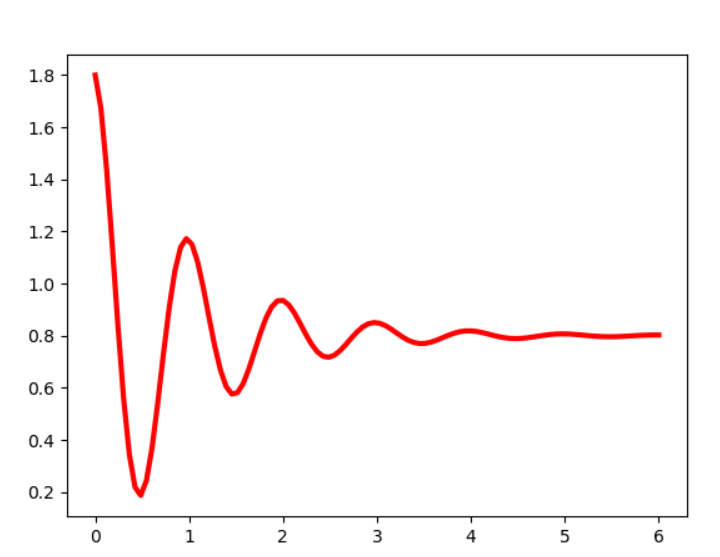
eg.绘制基本三角函数

import numpy as np
import matplotlib.pyplot as plt
x=np.linspace(0,6,100)
y=np.cos(2*np.pi*x)*np.exp(-x)+0.8
plt.plot(x,y,'k',color='r',linewidth=3,linestyle='-')
plt.show()

4.plt库的坐标轴设置函数

函数	描述
plt.axis('V','off','equal','scaled',tight','image')	获取设置轴属性的快捷方法
plt.xlim(xmin,xmax)	设置当前x轴取值范围
plt.ylim(ymin,ymax)	设置当前y轴取值范围
plt.xscale()	设置x轴缩放
plt.yscale()	设置y轴缩放
plt.autoscale()	自动缩放轴视图的数据
plt.text(x,y,s,fontdic,withdash)	为axes图轴添加注释
plt.thetagrids(angles,labels,fmt,frac)	设置极坐标网络theta的位置
plt.grid(on/off)	打开或者关闭坐标网络

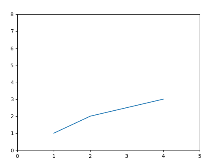
eg.(图如下：)

>>>import matplotlib.pyplot as plt
>>>plt.plot([1,2,4],[1,2,3])
>>>plt.axis()   #获取当前坐标轴范围
(0.85, 4.15, 0.9, 3.1)
>>>plt.axis([0,5,0,8])  #4个变量分别是[xmin,xmax,ymin,ymax]
[0, 5, 0, 8]
plt.show()

5.plt库的标签设置函数

函数	描述
plt.figlegend(handles,label,loc)	为全局绘图区域放置图注
plt.legend()	为当前坐标图放置图注
plt.xlabel()	设置当前x轴的标签
plt.ylabel()	设置当前y轴的标签
plt.xticks(array,'a','b','c')	设置当前x轴刻度位置的标签和值
plt.yticks(array,'a','b','c')	设置当前y轴刻度位置的标签和值
plt.clabel(cs,v)	为等值线图设置标签
plt.get_figlabels()	返回当前绘图区域的标签列表
plt.figtext(x,y,s,fontdic)	为全局绘图区域添加中心标题
plt.title()	设置标题
plt.suptitle()	为当前绘图区域添加中心标题
plt.text(x,y,s,fontdic,withdash)	为坐标轴添加注释
plt.annotate(note,xy,xytext,xycoords,textcoords,arrowprops)	用箭头在指定数据点创建一个注释或一段文本

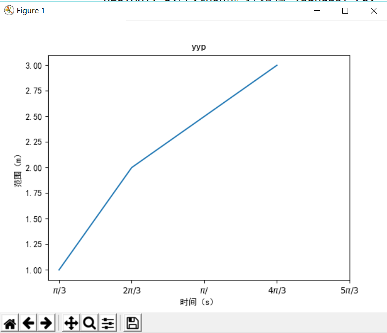
eg.带标签的坐标系

 eg.带标签的坐标系

import matplotlib.pyplot as plt
import matplotlib
matplotlib.rcParams['font.family']='SimHei'
matplotlib.rcParams['font.sans-serif']=['SimHei']
plt.plot([1,2,4],[1,2,3])
plt.title('yyp')     #坐标系标题
plt.xlabel('时间（s）')
plt.ylabel('范围（m）')
plt.xticks([1,2,3,4,5],[r'$pi/3$',r'$2pi/3$',r'$pi/$',r'$4pi/3$',r'$5pi/3$',])
plt.show()

6.plt库提供了三个区域填充函数，对绘图区域填充颜色

函数	描述
fill(x,y,color)	填充多边形
fill_between(x,y1,y2,where,color)	填充两条曲线围成的多边形
fill_betweenx(y,x1,x2,where,hold)	填充两条水平线之间的区域

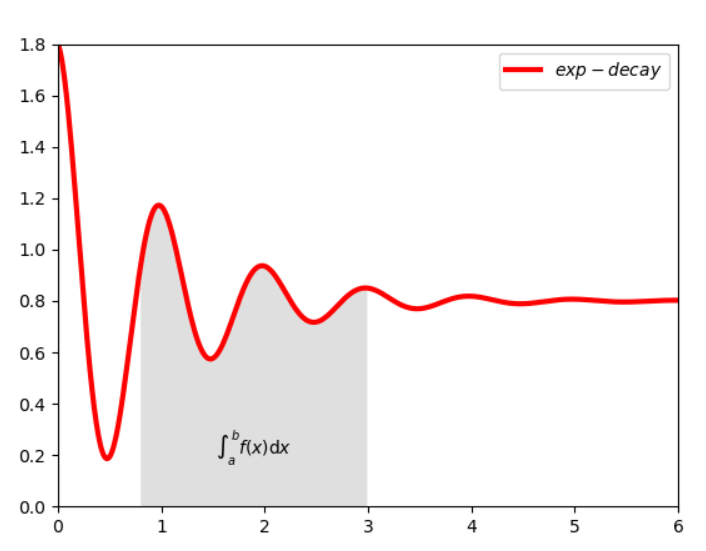
eg.带局部阴影的坐标系

import matplotlib.pyplot as plt
import numpy as np
x=np.linspace(0,10,1000)
y=np.cos(2*np.pi*x)*np.exp(-x)+0.8
plt.plot(x,y,'k',color='r',label="$exp-decay$",linewidth=3)
plt.axis([0,6,0,1.8])
ix=(x>0.8)&(x<3)
plt.fill_between(x,y,0,where=ix, 
                 facecolor='grey',alpha=0.25)
plt.text(0.5*(0.8+3),0.2,r"$int_a^b f(x)mathrm{d}x$",
         horizontalalignment='center')
plt.legend()
plt.show()

如图所示：

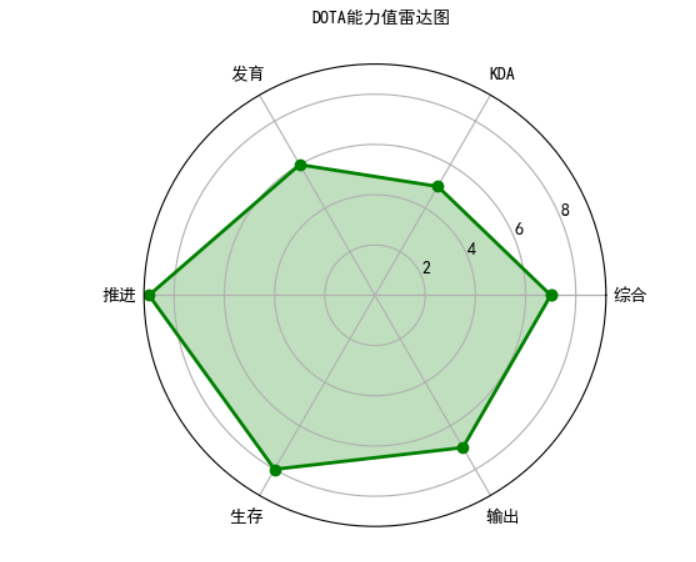
三、多级雷达图绘制[numpy、matplotlib综合运用]

 （1）

import numpy as np
import matplotlib.pyplot as plt
import matplotlib
matplotlib.rcParams['font.family']='simHei'
matplotlib.rcParams['font.sans-serif']=['simHei']   #显示中文
labels=np.array(['综合','KDA','发育','推进','生存','输出'])
nAttr=6
date=np.array([7,5,6,9,8,7])     #数据值
angles=np.linspace(0,2*np.pi,nAttr,endpoint=False)     #画出极坐标（角度）
date=np.concatenate((date,[date[0]]))
angles=np.concatenate((angles,[angles[0]]))
fig=plt.figure(facecolor="white")     #创建一个全局绘图区域，背景色为白色
plt.subplot(111,polar=True)     #创建子绘图区域，1*1网格，在第1个位置绘图（极坐标），
plt.plot(angles,date,'bo-',color='g',linewidth=2)  
plt.fill(angles,date,facecolor='g',alpha=0.25)    #填充颜色
plt.thetagrids(angles*180/np.pi,labels)   #设置极坐标网络 theta 的位置
plt.figtext(0.52,0.95,'DOTA能力值雷达图',ha='center')    #标签
plt.grid(True)   # 显示背景的网格线 
plt.savefig('dota_radar.JPG')  #保存图片
plt.show()

图如下：

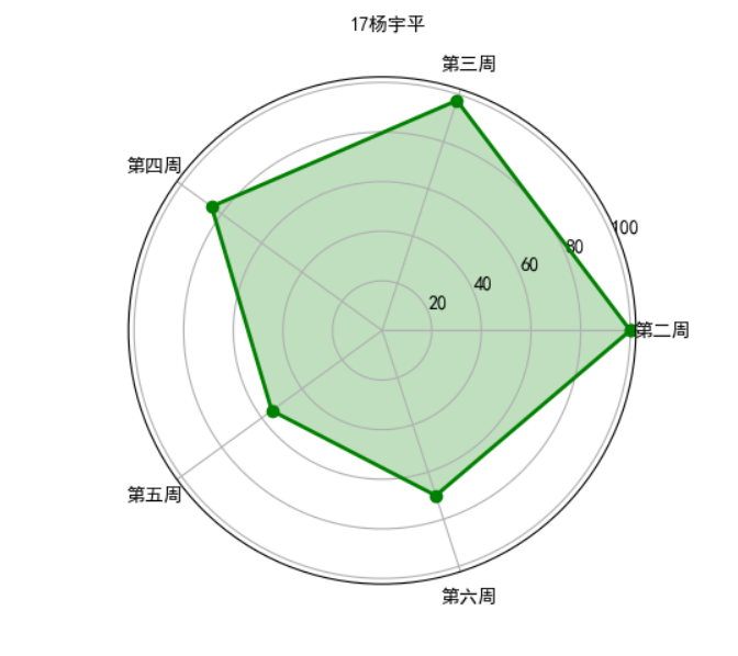
 （2）【作业： 把python123作业的成绩，画出雷达图，写上学号。】

import numpy as np
import matplotlib.pyplot as plt
import matplotlib
matplotlib.rcParams['font.family']='simHei'
matplotlib.rcParams['font.sans-serif']=['simHei']
labels=np.array(['第二周','第三周','第四周','第五周','第六周'])
nAttr=5
date=np.array([100,97.5,85,55,70])#数据值
angles=np.linspace(0,2*np.pi,nAttr,endpoint=False)
date=np.concatenate((date,[date[0]]))
angles=np.concatenate((angles,[angles[0]]))
fig=plt.figure(facecolor="white")
plt.subplot(111,polar=True)
plt.plot(angles,date,'bo-',color='g',linewidth=2)
plt.fill(angles,date,facecolor='g',alpha=0.25)
plt.thetagrids(angles*180/np.pi,labels)
plt.figtext(0.52,0.95,'17杨宇平',ha='center')
plt.grid(True)
plt.savefig('grade.JPG')
plt.show()

雷达图如图所示：

四、图像的手绘效果

这是一个使用  numpy  和  PLT  库提取图像特征形成手绘效果的实例

from PIL import Image
import numpy as np

a = np.asarray(Image.open("D:/Python练习/小宠物.jpg").convert('L')).astype('float')

depth = 10.                      # (0-100)
grad = np.gradient(a)             #取图像灰度的梯度值
grad_x, grad_y =grad               #分别取横纵图像梯度值
grad_x = grad_x*depth/100.
grad_y = grad_y*depth/100.
A = np.sqrt(grad_x**2 + grad_y**2 + 1.)
uni_x = grad_x/A
uni_y = grad_y/A
uni_z = 1./A

vec_el = np.pi/2.2                   # 光源的俯视角度，弧度值
vec_az = np.pi/4.                    # 光源的方位角度，弧度值
dx = np.cos(vec_el)*np.cos(vec_az)   #光源对x 轴的影响
dy = np.cos(vec_el)*np.sin(vec_az)   #光源对y 轴的影响
dz = np.sin(vec_el)              #光源对z 轴的影响

b = 255*(dx*uni_x + dy*uni_y + dz*uni_z)     #光源归一化
b = b.clip(0,255)

im = Image.fromarray(b.astype('uint8'))  #重构图像
im.show()

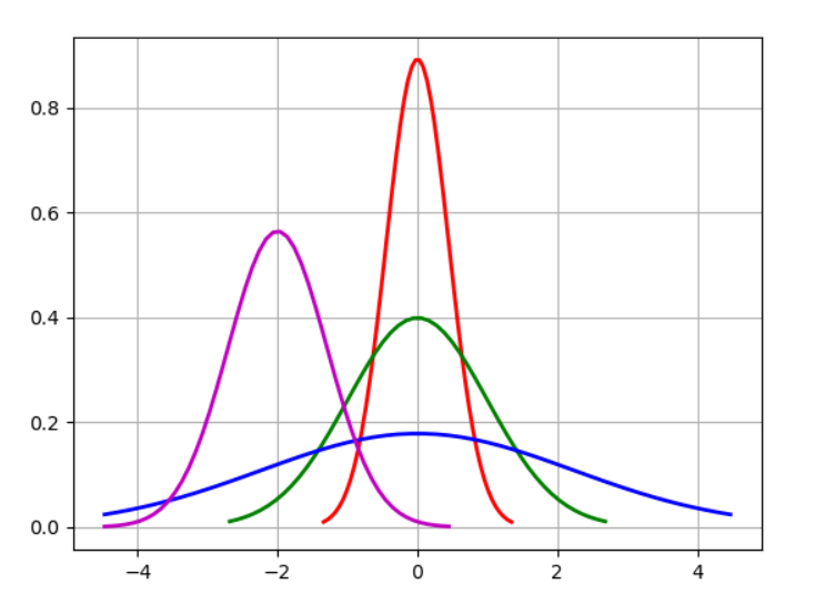
五、Python实现正态分布

绘制正态分布概率密度函数

# Python实现正态分布
# 绘制正态分布概率密度函数
import math
import numpy as np
import matplotlib.pyplot as plt
import matplotlib
u = 0     # 均值μ
u01 = -2
sig = math.sqrt(0.2)     # 标准差δ
sig01 = math.sqrt(1)
sig02 = math.sqrt(5)
sig_u01 = math.sqrt(0.5)
x = np.linspace(u - 3*sig, u + 3*sig, 50)
x_01 = np.linspace(u - 6 * sig, u + 6 * sig, 50)
x_02 = np.linspace(u - 10 * sig, u + 10 * sig, 50)
x_u01 = np.linspace(u - 10 * sig, u + 1 * sig, 50)
y_sig = np.exp(-(x - u) ** 2 /(2* sig **2))/(math.sqrt(2*math.pi)*sig)
y_sig01 = np.exp(-(x_01 - u) ** 2 /(2* sig01 **2))/(math.sqrt(2*math.pi)*sig01)
y_sig02 = np.exp(-(x_02 - u) ** 2 / (2 * sig02 ** 2)) / (math.sqrt(2 * math.pi) * sig02)
y_sig_u01 = np.exp(-(x_u01 - u01) ** 2 / (2 * sig_u01 ** 2)) / (math.sqrt(2 * math.pi) * sig_u01)
plt.plot(x, y_sig, "r-", linewidth=2)
plt.plot(x_01, y_sig01, "g-", linewidth=2)
plt.plot(x_02, y_sig02, "b-", linewidth=2)
plt.plot(x_u01, y_sig_u01, "m-", linewidth=2)
# plt.plot(x, y, 'r-', x, y, 'go', linewidth=2,markersize=8)
plt.grid(True)
plt.show()

图如下：