deep learning and neural networks--handwriting recongnization

use an algorithm to separate the letters from sentences. ( kind of classifier)

the architecture of neural networks:

　　input layer; hidden layer; output layer

different kinds of neural networks:

　　feedforward neural networks; recurrent neural networks; and so on

　　Usually, we use optimizer ( e.g. SGD Stochastic Gradient Descent in this chapter) to optimize/find a solution. As we all known, NNs is supervised learning. So we need to learn from the training dataset first, the we get our model from the data, then, test our result on the test dataset in the end.

traning dataset: MNIST data ( Modified NIST) comes in two parts: the first part contains 6000 images to be used as training data; the second part of the MNIST data set is 10000 images to be used as testing data.

notation x to denote a training input, it'll be regarded as a 28*28 = 784 dimensional vector as the image vector. And the corresponding output y = y(x) is a 10-dimensional vector. The element in y is either 0 or 1, and there will be only 1 in the vector y. ( e.g. if the input x is 6, if we recongnize the x correctly, then, the output y will be (0,0,0,0,0,0,1,0,0,0)^T ).

for each neuron, there are two parameters--weight and bias. Wj,k^l is weight of the lth connection the kth neuron ( right side) to the jth neron ( left side ). So after the formation the input x is z=w⋅x+b. Then, use the activation function in this chapter is sigmoid function to compute each output f(z) to decide which neuron to be fired.

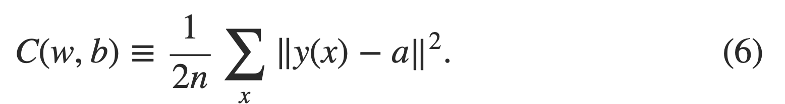
w denotes the collection of all weights in the network, b all the biases, n is the total number of training inputs, a is the vector of outputs from the network when x is input, and the sum is over all training inputs, x.

Why not try to maximize that number directly, rather than minimizing a proxy measure like the quadratic cost? The problem with that is that the number of images correctly classified is not a smooth function of the weights and biases in the network. For the most part, making small changes to the weights and biases won't cause any change at all in the number of training images classified correctly. That makes it difficult to figure out how to change the weights and biases to get improved performance. If we instead use a smooth cost function like the quadratic cost it turns out to be easy to figure out how to make small changes in the weights and biases so as to get an improvement in the cost.

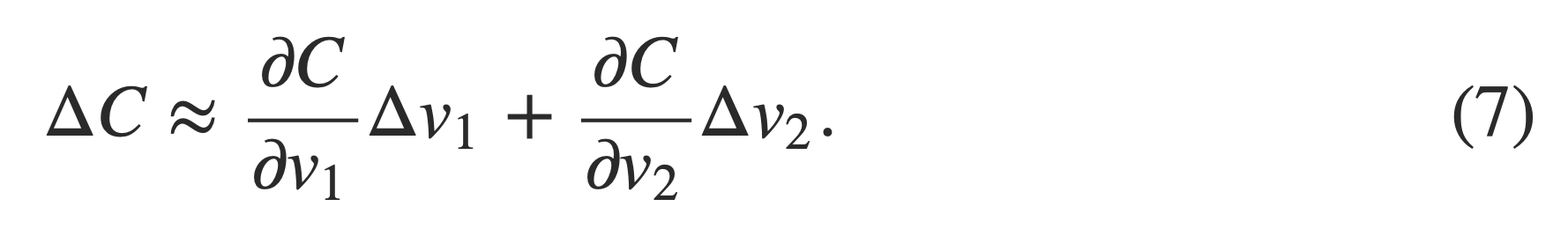
The cost function C changes as follows, then, we need to choose Δv₁, Δv₂ to make (7) negative.

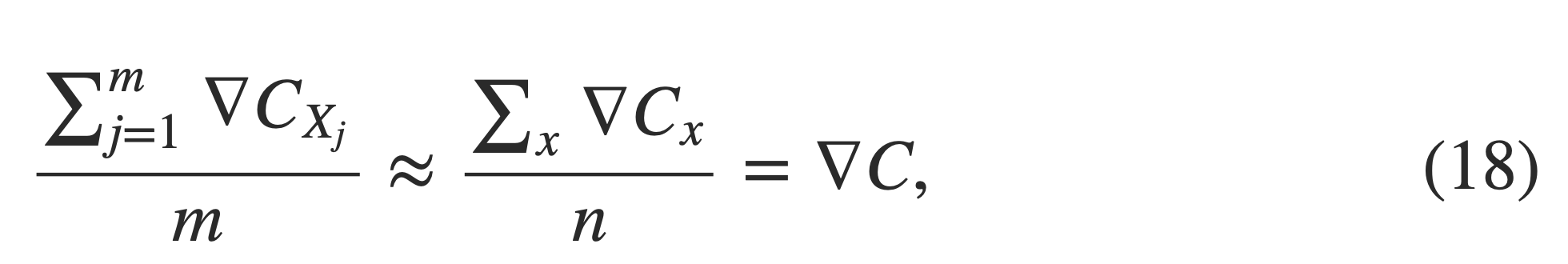
An idea called stochastic gradient descent can be used to speed up learning. The idea is to estimate the gradient ∇Cby computing ∇Cx for a small sample of randomly chosen training inputs. By averaging over this small sample it turns out that we can quickly get a good estimate of the true gradient ∇C∇C, and this helps speed up gradient descent, and thus learning.

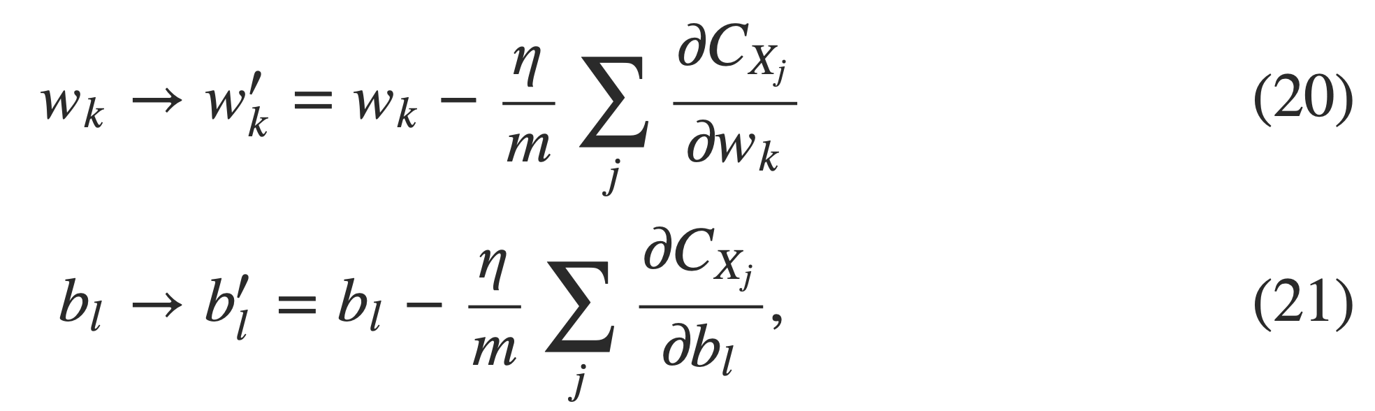
Then stochastic gradient descent works by picking out a randomly chosen mini-batch of training inputs, and training with those, ( In other words, use backpropagation to update w,b in each mini-batch) Then we get the final set of weights and biases of the neural network as the result

# %load network.py

"""
network.py
~~~~~~~~~~
IT WORKS

A module to implement the stochastic gradient descent learning
algorithm for a feedforward neural network.  Gradients are calculated
using backpropagation.  Note that I have focused on making the code
simple, easily readable, and easily modifiable.  It is not optimized,
and omits many desirable features.
"""

#### Libraries
# Standard library
import random

# Third-party libraries
import numpy as np

class Network(object):

    def __init__(self, sizes):
        """The list ``sizes`` contains the number of neurons in the
        respective layers of the network.  For example, if the list
        was [2, 3, 1] then it would be a three-layer network, with the
        first layer containing 2 neurons, the second layer 3 neurons,
        and the third layer 1 neuron.  The biases and weights for the
        network are initialized randomly, using a Gaussian
        distribution with mean 0, and variance 1.  Note that the first
        layer is assumed to be an input layer, and by convention we
        won't set any biases for those neurons, since biases are only
        ever used in computing the outputs from later layers."""
        self.num_layers = len(sizes)
        self.sizes = sizes
        self.biases = [np.random.randn(y, 1) for y in sizes[1:]]
        self.weights = [np.random.randn(y, x)
                        for x, y in zip(sizes[:-1], sizes[1:])]

    def feedforward(self, a):
        """Return the output of the network if ``a`` is input."""
        for b, w in zip(self.biases, self.weights):
            a = sigmoid(np.dot(w, a)+b)
        return a

    def SGD(self, training_data, epochs, mini_batch_size, eta,
            test_data=None):
        """Train the neural network using mini-batch stochastic
        gradient descent.  The ``training_data`` is a list of tuples
        ``(x, y)`` representing the training inputs and the desired
        outputs.  The other non-optional parameters are
        self-explanatory.  If ``test_data`` is provided then the
        network will be evaluated against the test data after each
        epoch, and partial progress printed out.  This is useful for
        tracking progress, but slows things down substantially."""

        training_data = list(training_data)
        n = len(training_data)

        if test_data:
            test_data = list(test_data)
            n_test = len(test_data)

        for j in range(epochs):
            random.shuffle(training_data)
            mini_batches = [
                training_data[k:k+mini_batch_size]
                for k in range(0, n, mini_batch_size)]
            for mini_batch in mini_batches:
                self.update_mini_batch(mini_batch, eta)
            if test_data:
                print("Epoch {} : {} / {}".format(j,self.evaluate(test_data),n_test));
            else:
                print("Epoch {} complete".format(j))

    def update_mini_batch(self, mini_batch, eta):
        """Update the network's weights and biases by applying
        gradient descent using backpropagation to a single mini batch.
        The ``mini_batch`` is a list of tuples ``(x, y)``, and ``eta``
        is the learning rate."""
        nabla_b = [np.zeros(b.shape) for b in self.biases]
        nabla_w = [np.zeros(w.shape) for w in self.weights]
        for x, y in mini_batch:
            delta_nabla_b, delta_nabla_w = self.backprop(x, y)
            nabla_b = [nb+dnb for nb, dnb in zip(nabla_b, delta_nabla_b)]
            nabla_w = [nw+dnw for nw, dnw in zip(nabla_w, delta_nabla_w)]
        self.weights = [w-(eta/len(mini_batch))*nw
                        for w, nw in zip(self.weights, nabla_w)]
        self.biases = [b-(eta/len(mini_batch))*nb
                       for b, nb in zip(self.biases, nabla_b)]

    def backprop(self, x, y):
        """Return a tuple ``(nabla_b, nabla_w)`` representing the
        gradient for the cost function C_x.  ``nabla_b`` and
        ``nabla_w`` are layer-by-layer lists of numpy arrays, similar
        to ``self.biases`` and ``self.weights``."""
        nabla_b = [np.zeros(b.shape) for b in self.biases]
        nabla_w = [np.zeros(w.shape) for w in self.weights]
        # feedforward
        activation = x
        activations = [x] # list to store all the activations, layer by layer
        zs = [] # list to store all the z vectors, layer by layer
        for b, w in zip(self.biases, self.weights):
            z = np.dot(w, activation)+b
            zs.append(z)
            activation = sigmoid(z)
            activations.append(activation)
        # backward pass
        delta = self.cost_derivative(activations[-1], y) * 
            sigmoid_prime(zs[-1])
        nabla_b[-1] = delta
        nabla_w[-1] = np.dot(delta, activations[-2].transpose())
        # Note that the variable l in the loop below is used a little
        # differently to the notation in Chapter 2 of the book.  Here,
        # l = 1 means the last layer of neurons, l = 2 is the
        # second-last layer, and so on.  It's a renumbering of the
        # scheme in the book, used here to take advantage of the fact
        # that Python can use negative indices in lists.
        for l in range(2, self.num_layers):
            z = zs[-l]
            sp = sigmoid_prime(z)
            delta = np.dot(self.weights[-l+1].transpose(), delta) * sp
            nabla_b[-l] = delta
            nabla_w[-l] = np.dot(delta, activations[-l-1].transpose())
        return (nabla_b, nabla_w)

    def evaluate(self, test_data):
        """Return the number of test inputs for which the neural
        network outputs the correct result. Note that the neural
        network's output is assumed to be the index of whichever
        neuron in the final layer has the highest activation."""
        test_results = [(np.argmax(self.feedforward(x)), y)
                        for (x, y) in test_data]
        return sum(int(x == y) for (x, y) in test_results)

    def cost_derivative(self, output_activations, y):
        """Return the vector of partial derivatives partial C_x /
        partial a for the output activations."""
        return (output_activations-y)

#### Miscellaneous functions
def sigmoid(z):
    """The sigmoid function."""
    return 1.0/(1.0+np.exp(-z))

def sigmoid_prime(z):
    """Derivative of the sigmoid function."""
    return sigmoid(z)*(1-sigmoid(z))