- Generalized Linear Models
In the regression problem, we had y|x;θ ~ N(μ, σ2), and in the classification one, y|x;θ ~ Bernoulli(Φ), for some appropriate definitions of μ and Φ as functions of x and θ. In this section we will show that both of these methods are special cases of a broader family of models, called Generalized Linear Models(GLMs). We will also show how other models in GLM family can be derived and applied to other classification and regerssion problems.
- The exponential family
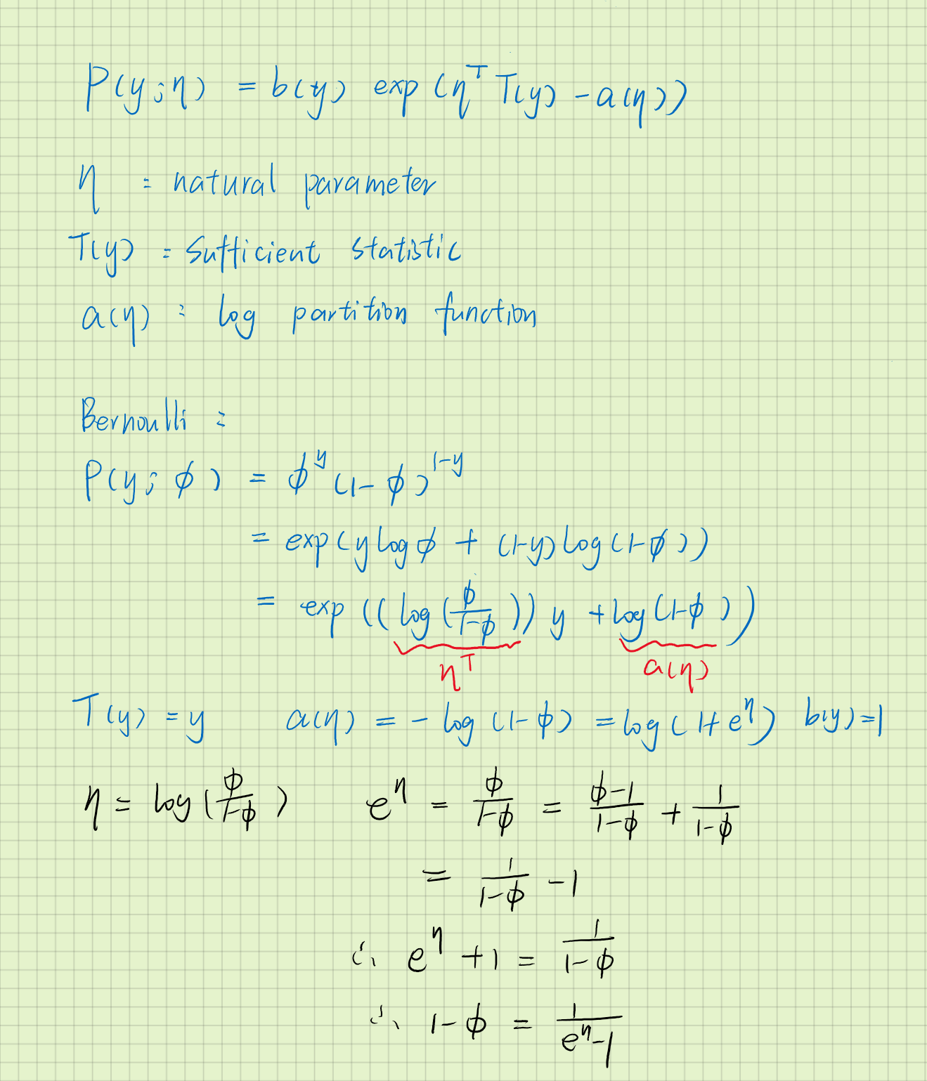
p(y; η) = b(y)exp(ηTT(y) - a(η))
Here, η is called the natural parameter(also called the canonical parameter) of the distribution; T(y) is suffcient statistic (for the distributions we consider, it willl often be the case that T(y) = y); and a(η) is the log partition function. The quantity e-a(η) essentially plays the role of a normalization constant, that makes sure the distribution p(y; η) sums/integrates over y to 1.
The Bernoulli and Gaussian distributions are examples of exponential family distributions.
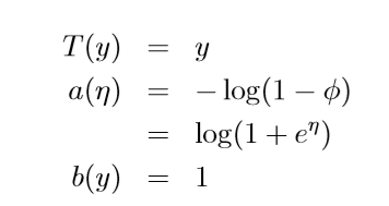
- The Bernoulli distribution with mean Φ, written Bernoulli(Φ), specifies a distribution over y ∈ { 0, 1}, so that


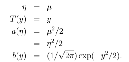
- Gaussian distribution. Recall that, when deriving linear regerssion, the value of σ2 had no effect on our final choice of θ and hθ(x). Thus we can choose an arbitrary value for σ2 without changing anything. To simplify the derivation below, let's set σ2 = 1. We then have:


- Constructing GLMs(Generalized Linear Models)
Consider a classification or regression problem where we would like to predict the value of some random variable y as a function of x. To derive a GLM for this problem, we will make the following three assumptions about the conditional distribution of y given x and about our model:
- y|x;θ ~ ExponentialFamily(η). I.e., given x and θ, the distribution of y follows some exponential family distribution, with parameter η.
- Given x, our goal is to predict the expected value of T(y) given x. In most of our examples, we will have T(y) = y, so this means we would like the prediction h(x) output by our learned hypothesis h to satisfy h(x) = E[y|x]
- The natural parameter η and the inputs x are related linearly: η = θTx.
The third of these assumptions might seem the least well justified of the above, and it might be better thought of as a "design choice" in our recipe for designing GLMs, rather than as an assumption per se.