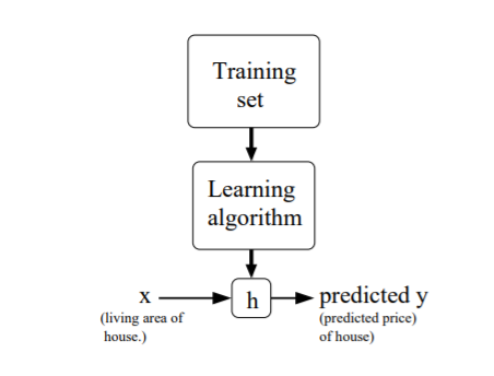
- the process of supervised learning
given dataset with labels then learn the hypothesis/predict function h: x->y through learning algorithm. When the target variable we try to predict is continuous, we call it regression problem. Whrn the target variable we try to predict is discrete, we call it classification problem.

- Linear regression
e.g. prediction of houses' price, give living area x1, number of bedrooms x2
hθ(x) = θ0 + θ1x1 + θ2x2
θi's are parameters/weight value, for simplicity, we can write in vectors as
h(x) = sum(θixi ) = θTx
to get parameter θ we define the cost function:
J(θ) = 1/2sum(hθ(x(i)) - y(i))2
-
- LMS algorithm (Least Mean Squares)
-
consider gradient descent algorithm(find local minimum), which starts with some initial θ, and repeatedly performs the update:(repeat until convergence)
θj := θj - α*∂J(θ)/∂θj
∂J(θ)/∂θj = (hθ(x) - y)*xj
-
- The normal equations
- instead of iterative algorithm, minimize J(θ) by explicitly taking its derivatives with respect to the θj' s, and setting them to zero.
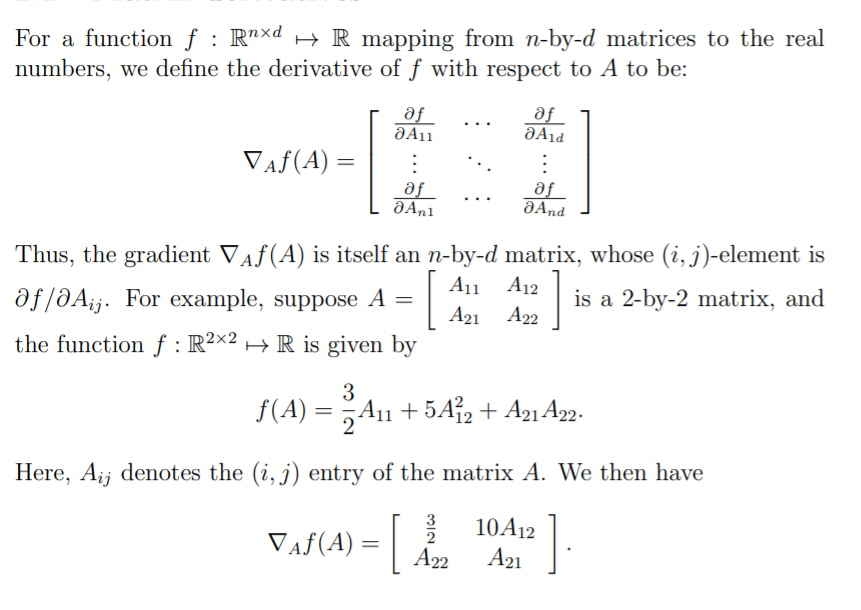
- Matrix derivative(click for more info on WIKI)
- LMS algorithm (Least Mean Squares)
-
- Probabilistic interpretation( of least squares)
- Assume that the target variables and the inputs are related via the equation y(i) = θTx(i) + ε(i), where ε(i) is an error term that captures either unmodeled effects ( such as if there are some features very pertinent相关的特征to predict housing price, but that we'd left out of the regression), or random nosie.
- further assume that the ε(i) are distributed IID( independently and identically distribution)accroding to Gaussian distribution( also called Normal distribution) . I.e., the density of ε(i) is given by

-
-
- Then, construct likelihood function:

- Next, get log likelihood l(θ)

- Hence, maximizing l(θ) gives the same answer as minimizing J(θ) below, the original least-square function

- Then, construct likelihood function:
-
